Matlab Tutorial : Vectors (Arrays) with Audio Files

In this chapter, we'll learn more about the vectors (arrays) while we playing with audio files. Our primary focus is on vectors but not on audio. Regarding audio, we'll have a chance to get more deep in later chapters.

First, we need to read in the audio files using wavread() into arrays:

>> mantle = wavread('C:\SOUND\Clock_mantle.wav');
>> drum = wavread('C:\SOUND\Bogos_Drum.wav');
>> flag = wavread('C:\SOUND\FlagRaising.wav');
>> taps = wavread('C:\SOUND\Taps.wav');

The files are available:

1. Clock_mantle.wav
2. Bogos_Drum.wav
3. FlagRaising.wav
4. Taps.wav

Let's see what's in there:

>> mantle
         0
   -0.0000
         0
   -0.0000
         0
   -0.0000
         0
   -0.0001
   -0.0003
    ...
    0.0006
   -0.0009
    0.0002
    0.0018

The signal is quite long, and we can check how long it is:

>> length(mantle)
ans =
      302697

The audio sampling rate is 22050 (unfortunately, it's not CD quality 44.1 kHz), and we can calculate the duration:

>> dur = length(mantle)/22050
dur =
   13.7278

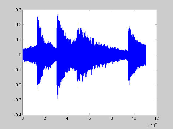
So, the duration is about 13 seconds. If we want to grab some portion (5-10 sec), we can use colon (':') like this:

>> rate = 22050;
>> m_seg = mantle(rate*5:rate*10);

We can plot the signal:

>> plot(m_seg)

We can also play back using Matlab's built in function sound():

>> sound(m_seg, rate);

We can play it with higher rage, and if we double it or play it half of the recording rate:

>> sound(m_seg, rate*2);
>> sound(m_seg, rate*0.5);

We may want to play with another sound and get more info while reading it in.

>> [d, fs] = wavread('C:\SOUND\Bogos_Drum.wav');
>> fs
fs =
       11025

This time, we get the sample rate, $f_s$ as well.

Plot the audio:

>> plot(d);

Unlike the previous audio (mantle), now we have two channels:

So, we need to check the size:

>> size(d)
ans =
       88600           2

How about the previous one:

>> size(mantle)
ans =
      302697           1

Indeed! We had only one channel with the previous audio sample.

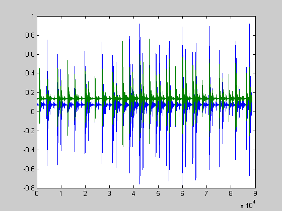
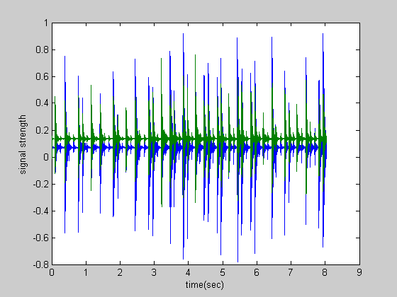
We want to separate the channels into two: left and right. Also, we want to use time as x-axis. The following script does it all:

left = d(:,1);
right = d(:,2);

time = (1/fs)*length(d);
t = linspace(0, time, length(left));
plot(t,left, t, right);
xlabel('time(sec)');
ylabel('signal strength');

Let's listen to the audio both in mono and in stereo:

>> sound(left, fs);     # mono
>> sound(right, fs);    # mono
>> sound(d, fs);        # stereo

Let's check the array:

>> left(10:15)
ans =
    0.0023
   -0.0052
    0.0231
    0.0658
    0.0559
    0.0604

>> right(10:15)
ans =
    0.0053
   -0.0115
    0.0527
    0.1541
    0.1322
    0.1362

>> d(10:15,:)
ans =
    0.0023    0.0053
   -0.0052   -0.0115
    0.0231    0.0527
    0.0658    0.1541
    0.0559    0.1322
    0.0604    0.1362

As we see, each column of d are composed of left and right column vector. Then, how we make d from the two column vectors?

d_new = [left ; right]?

The operation just append the right to the end of left, which makes it 2*length(left) x 1 matrix:

>> d_new = [left;right];
>> size(d_new)
ans =
      177200           1

>> size(left)
ans =
       88600           1

The answer is this:

>> d_stereo = [left right];
>> size(d)
ans =
       88600   

The audio is too short, and we want to hear it repeatedly. What should we do?

>> d_repeat = [d_stereo ; d_stereo; d_stereo];
>> sound(d_repeat, fs);

We can reverse a column vector using flip-upside-down, flipud():

>> cvec = [1;2;3;4;5]
cvec =
     1
     2
     3
     4
     5

>> rev_cvec = flipud(cvec)
rev_cvec =
     5
     4
     3
     2
     1

Using this reverse, we can play an audio reverse:

>> d_reverse = flipud(d);
>> sound(d_reverse, fs);