Convolution - Impulse Response of LTI / LSI system 2020

In this chapter, we'll learn linear time-invariant(LTI)/linear shift-invariant(LSI) system. They are basically equivalent: the linear time invariant systems refers to an analog system and shift-invariant system refers to a discrete-time system.
Because the system is linear, whenever we express an input as a sum of simpler signals, the output is equal to the super position of the outputs that we got when we apply each input. The shift-invariant is the same as time invariant: if we delay the input, the output that we get is the original input to the signal that wasn't delayed. No matter what delay we pick, the system doesn't change with time.
As will be describe below, there are two key attributes in LSI/LTI system which make the system more friendly. The linear and invariant properties of the system allow us to handle the system in a straight forward manner: "the output of the system is simply the convolution of the input to the system with the system's impulse response."
The impulse response and frequency response are two attributes that are useful for characterizing LTI/LSI systems. They provide two different ways of calculating what the system's output will be for a given input signal.
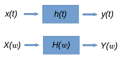
As shown in the diagram, the system $h(t)$ maps its input signal $x(t)$ to a corresponding output signal $y(t)$. Let's look at the key two attributes in detail:
- linear:
We can do superposition. Linearity means that the sum of signals is that the input of a linear system. So, the system can process each signal separately, and add up the processed signals:: if $x_1(t)$ maps to an output of $y_1(t)$ and $x_2(t)$ maps to an output of $y_2(t)$, then for all values of $a_1$ and $a_2$,
$$ h\{a_1 x_1(t) + a_2 x_2(t)\} = a_1 y_1(t) + a_2 y_2(t) $$
- time-invariant
System's characteristics do not change with time. Also, spatial invariance means that, It is irrelevant where the origin of the coordinate system is located.
If we add a delay to the input signal, then we simply add the same delay to the output. For an input signal $x(t)$ that maps to an output signal $y(t)$, then for all values of $\tau$,
$$ h\{x(t - \tau)\} = y(t - \tau) $$
These characteristics allow the operation of the system to be characterized using its impulse and frequency responses. They provide two perspectives on the system that can be used in different contexts.
The impulse is referred to a short-duration time-domain signal. For continuous-time systems, this is the Dirac delta function $\delta(t)$, while for discrete-time systems, the Kronecker delta function $\delta[n]$ is typically used. A system's impulse response (often annotated as $h(t)$ for continuous-time systems or $h[n]$ for discrete-time systems) is defined as the output signal that results when an impulse is applied to the system input.
Why is this important and useful?
That's because the theory of the convolution integral will give us a method of determining the response of a system to an input once we know its unit impulse response!.
In other words, it allows us to predict what the system's output will look like. Thanks to the linearity and time-invariance properties, once we can decompose the system's input signal, then the output is equal to the sum of the system outputs for each of those components. What if we could decompose our input signal into a sum of scaled and time-shifted impulses? Then, the output would be equal to the sum of copies of the impulse response, scaled and time-shifted in the same way.
For discrete-time systems, this is possible, because you can write any signal $x[n]$ as a sum of scaled and time-shifted Kronecker delta functions:
$$ x[n] = \sum_{k=0}^{\infty} x[k] \delta[n - k] $$
Each term in the sum is an impulse scaled by the value of $x[n]$ at that time instant.
What would we get if we passed $x[n]$ through an LTI/LSI system to yield $y[n]$?
Each scaled and time-delayed impulse that we put in yields a scaled and time-delayed copy of the impulse response at the output:
$$ y[n] = \sum_{k=0}^{\infty} x[k] h[n-k] $$
where $h[n]$ is the system's impulse response. The above equation is the convolution theorem for discrete-time systems. That is, for any signal $x[n]$ that is input to a system, the system's output $y[n]$ is equal to the discrete convolution of the input signal and the system's impulse response.
For continuous-time systems, the above straightforward decomposition isn't possible in a strict mathematical sense (the Dirac delta has zero width and infinite height), but at an engineering level, it's an approximate, intuitive way of looking at the problem. A similar convolution theorem holds for these systems:
$$ y(t) = \int_{-\infty}^{\infty} x(\tau) h(t - \tau) d\tau $$
where, again, $h(t)$ is the system's impulse response. There are a number of ways of deriving this relationship.
The impulse response is useful because it allows us to calculate the output of these systems for any input signal: the output is simply the input signal convolved with the impulse response function.
One of the most important operations in signal processing is the convolution performed by LSI systems.
LSI systems are uniquely defined by their impulse response: the response of the system to a two-dimensional impulse. The output of an LSI system to any input is simply the convolution of the input with the impulse response of the system.
$$ y[n] = \sum_{k=0}^{\infty} x[k] h[n-k] $$Let us derive now an expression for 2-D convolution. Let's put any signal and get the sum of shifted deltas. These deltas are shifted at all possible pixel locations in an image. The height of the delta, $x(k_1,k_2)$, could be just the value of the signal at the location of the delta, or the intensity values of these pixels.
As an example, let's make a signal and decompose it.
$$ x(n_1,n_2) = \sum_{k_1=-\infty}^{\infty} \sum_{k_2=-\infty}^{\infty} x(k_1,k_2) \delta(n_1-k_1,n_2-k_2) $$The picture below shows how the signal $x(n_1,n_2)$ can be decomposed.

The signal in the picture above has only four pixels with values of 1, 2, 3, and 4. We can clearly see that we can decompose the signal as a signal like that, so it's a delta at the origin, with height two, plus at $n_1=-1$ with a value of 1, at $n_1 = 1$ with a value of 3, and the last one at $n_2 = 1$ with a value of 4.
Now, we can get the response $y(n_1,n_2)$:
$$ y(n_1,n_2) = T[x(n_1,n_2)] = T \left[\sum_{k_1=-\infty}^{\infty} \sum_{k_2=-\infty}^{\infty} x(k_1,k_2) \delta(n_1-k_1,n_2-k_2) \right] $$Because our system is linear, the output of the system is going to be the sum of the weighted individual outputs. So the weights are $k_1$, $k_2$, and the output is $T$ with $\delta$, shifted $\delta$s at the input.
$$ y(n_1,n_2) = \sum_{k_1=-\infty}^{\infty} \sum_{k_2=-\infty}^{\infty} x(k_1,k_2) T [ \delta(n_1-k_1,n_2-k_2) ] $$We know the response of the system to a $\delta$. Yes, that's the impulse response we denoted by $h$.
Since the system is spatially invariant and the input($\delta$) is shifted, the output $h$ is going to be shifted by the same amount. So, the output would be shifted by $k_1$, $k_2$. So, this is the of sum of the convolution: convolution of $x$ with $h$.
$$ y(n_1,n_2) = \sum_{k_1=-\infty}^{\infty} \sum_{k_2=-\infty}^{\infty} x(k_1,k_2) h(n_1-k_1,n_2-k_2) = x(n_1,n_2)*h(n_1,n_2) $$Let's walk through the convolution of two simple signals: $x(n_1,n_2)$ and $h(n_1,n_2)$.
$$ y(n_1,n_2) = x(n_1,n_2) * h(n_1,n_2) = \sum_{k_1=\infty}^{\infty} \sum_{k_2=\infty}^{\infty} x(k_1,k_2) h(n_1-k_1,n_2-k_2) $$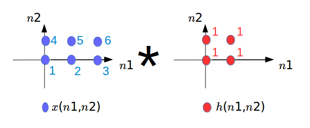
Notice that we have to rename the independant axis from $n_1$, $n_2$ to $k_1$, $k_2$ for both $x$ and $h$. For $h$, however, we see the shift of it with respect to the horizontal and the vertical axis. Then, we shift this reflected version by amounts $n_1$, $n_2$. For each shift, we find the product of $h$ with $x$, and we sum up this product for $k_1$ and $k_2$ to infinity.
So, for this particular shift we'll find the output, $y(n_1$, $n_2)$. We have to perform all possible shifts in order to find $y$ in all possible pixels locations, $n_1$ and $n_2$.
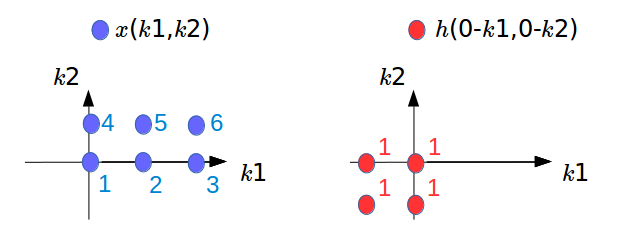
Note that now we have $x(k_1,k_2)$ and $h(k_1,k_2)$, but we reflected it with respect to the vertical and horizontal axis.
The picture below shows the case when we superimpose the signals:
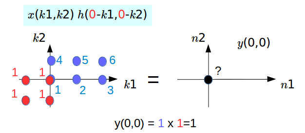
For the shift in the picture above, we know $h$ is sifted by $(0,0)$. Now we're going to find the product of the two signals, and we'll sum it up to find the value of y at $(0,0)$.
We see that for this case, the overlap is only at one pixel location. So, we have $y(0,0)=1 \times 1 = 1$.
For the next one, we have two overlaps:
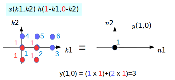
The same to the next ones:
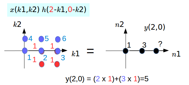
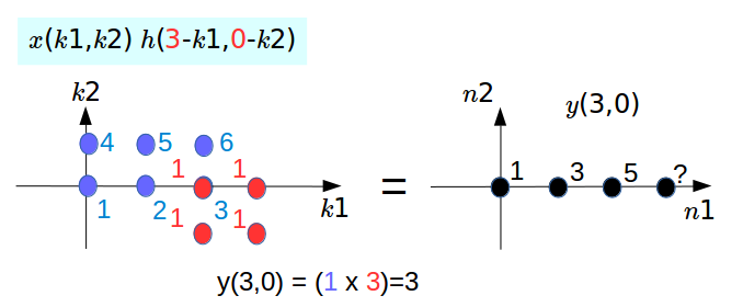
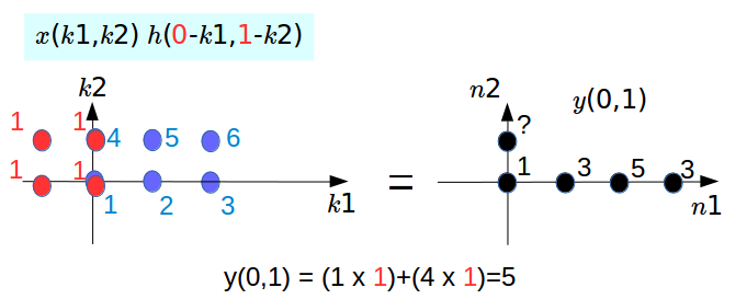
The same process for the rest, and the picture below is the last step.
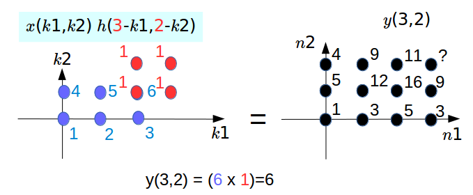
Any other shift of $h$ will result in no overlap between $x$ and the shifted $h$, and therefore the value of $y$ is going to be equal to 0.
This is the final result for the convolution:
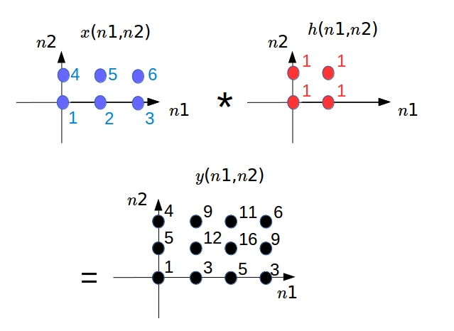
We see that the signal $y$ is the result of the convolution of $x$ with $h$.
In image processing, many filter operations are applied to an image by performing a special operation called convolution with a matrix called a kernel.
Kernels are typically 3x3 square matrices, although kernels of size 2x2, 4x4, and 5x5 are sometimes used. The values stored in the kernel directly relate to the results of applying the filter, and filters are characterized solely by their kernel matrix.
For more applications of convolution and kernel matrix to Image processing, please visit my other OpenCV tutorials.
- impulse response
- frequency response
- What is meant by a system's âimpulse responseâ and âfrequency response?â
- Fundamentals of Digital Image and Video Processing
Ph.D. / Golden Gate Ave, San Francisco / Seoul National Univ / Carnegie Mellon / UC Berkeley / DevOps / Deep Learning / Visualization