Machine Learning : k-Means Clustering I

The k-Means Clustering finds centers of clusters and groups input samples around the clusters.
k-Means Clustering is a partitioning method which partitions data into k mutually exclusive clusters, and returns the index of the cluster to which it has assigned each observation. Unlike hierarchical clustering, k-means clustering operates on actual observations (rather than the larger set of dissimilarity measures), and creates a single level of clusters. The distinctions mean that k-means clustering is often more suitable than hierarchical clustering for large amounts of data.
The following description for the steps is from wiki - K-means_clustering.
Step 1
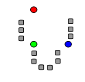
k initial "means" (in this case k=3) are randomly generated within the data domain.
Step 2
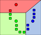
k clusters are created by associating every observation with the nearest mean. The partitions here represent the Voronoi diagram generated by the means.
Step 3
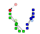
The centroid of each of the k clusters becomes the new mean.
Step 4
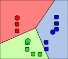
Steps 2 and 3 are repeated until convergence has been reached.
In OpenCV, we use cv.KMeans2(() and it's defined like this:
cv2.kmeans(data, K, criteria, attempts, flags[, bestLabels[, centers]])
The parameters are:
- data : Data for clustering.
- nclusters(K) K : Number of clusters to split the set by.
- criteria : The algorithm termination criteria, that is, the maximum number of iterations and/or the desired accuracy. The accuracy is specified as criteria.epsilon. As soon as each of the cluster centers moves by less than criteria.epsilon on some iteration, the algorithm stops.
- attempts : Flag to specify the number of times the algorithm is executed using different initial labellings. The algorithm returns the labels that yield the best compactness (see the last function parameter).
- flags :
- KMEANS_RANDOM_CENTERS - selects random initial centers in each attempt.
- KMEANS_PP_CENTERS - uses kmeans++ center initialization by Arthur and Vassilvitskii.
- KMEANS_USE_INITIAL_LABELS - during the first (and possibly the only) attempt, use the user-supplied labels instead of computing them from the initial centers. For the second and further attempts, use the random or semi-random centers. Use one of KMEANS_*_CENTERS flag to specify the exact method.
- centers : Output matrix of the cluster centers, one row per each cluster center.
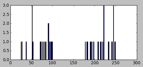
In this section, we'll play with a data set which has only one feature. The data is one-dimensional, and clustering can be decided by one parameter.
We generated two groups of random numbers in two separated ranges, each group with 25 numbers as shown in the picture below:
The code:
import numpy as np
import cv2
from matplotlib import pyplot as plt

x = np.random.randint(25,100,25)   # 25 randoms in (25,100)
y = np.random.randint(175,250,25)  # 25 randoms in (175,250)
z = np.hstack((x,y))               # z.shape : (50,)
z = z.reshape((50,1))              # reshape to a column vector
z = np.float32(z)
plt.hist(z,256,[0,256])
plt.show()
Now, we're going to apply cv2.kmeans() function to the data with the following parameters:
# Define criteria = ( type, max_iter = 10 , epsilon = 1.0 )
criteria = (cv2.TERM_CRITERIA_EPS + cv2.TERM_CRITERIA_MAX_ITER, 10, 1.0)

# Set flags
flags = cv2.KMEANS_RANDOM_CENTERS

# Apply KMeans
compactness,labels,centers = cv2.kmeans(z,2,None,criteria,10,flags)
In the code, the criteria means whenever 10 iterations of algorithm is ran, or an accuracy of epsilon = 1.0 is reached, stop the algorithm and return the answer.
Here are the meanings of the return values from cv2.kmeans() function:
- compactness : It is the sum of squared distance from each point to their corresponding centers.
- labels : This is the label array where each element marked '0','1',.....
- centers : This is array of centers of clusters.
For the current case, it gives us centers as:
centers: [[ 72.08000183] [ 217.03999329]]
Here is the final code for 1-D data:
import numpy as np
import cv2
from matplotlib import pyplot as plt

x = np.random.randint(25,100,25)   # 25 randoms in (25,100)
y = np.random.randint(175,250,25)  # 25 randoms in (175,250)
z = np.hstack((x,y))               # z.shape : (50,)
z = z.reshape((50,1))              # reshape to a column vector
z = np.float32(z)


# Define criteria = ( type, max_iter = 10 , epsilon = 1.0 )
criteria = (cv2.TERM_CRITERIA_EPS + cv2.TERM_CRITERIA_MAX_ITER, 10, 1.0)

# Set flags
flags = cv2.KMEANS_RANDOM_CENTERS

# Apply KMeans
compactness,labels,centers = cv2.kmeans(z,2,None,criteria,10,flags)

print('centers: %s' %centers)

A = z[labels==0]
B = z[labels==1]

# initial plot
plt.subplot(211)
plt.hist(z,256,[0,256])

# Now plot 'A' in red, 'B' in blue, 'centers' in yellow
plt.subplot(212)
plt.hist(A,256,[0,256],color = 'r')
plt.hist(B,256,[0,256],color = 'b')
plt.hist(centers,32,[0,256],color = 'y')

plt.show()
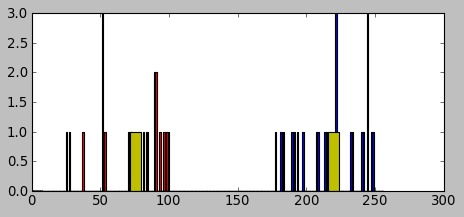
We can see the data has been clustered: A's centroid is 72 and B's centroid is 217 which was one of the outputs from the cv2.kmeans() function.
Ph.D. / Golden Gate Ave, San Francisco / Seoul National Univ / Carnegie Mellon / UC Berkeley / DevOps / Deep Learning / Visualization