Image Edge Detection : Sobel and Laplacian

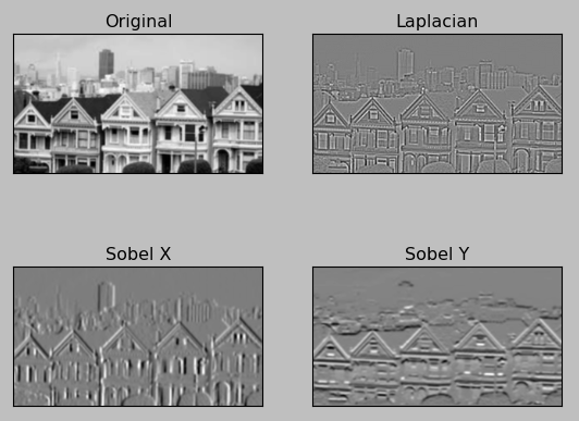
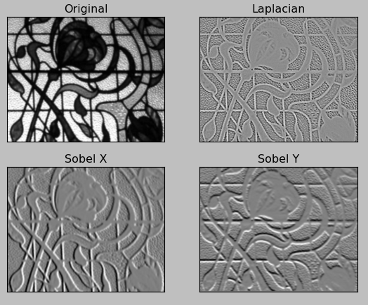
Edge detection is one of the fundamental operations when we perform image processing. It helps us reduce the amount of data (pixels) to process and maintains the structural aspect of the image. We're going to look into two commonly used edge detection schemes - the gradient (Sobel - first order derivatives) based edge detector and the Laplacian (2nd order derivative, so it is extremely sensitive to noise) based edge detector. Both of them work with convolutions and achieve the same end goal - Edge Detection.

Sobel edge detector is a gradient based method based on the first order derivatives. It calculates the first derivatives of the image separately for the X and Y axes.

The operator uses two 3X3 kernels which are convolved with the original image to calculate approximations of the derivatives - one for horizontal changes, and one for vertical. The picture below shows Sobel Kernels in x-dir and y-dir:

For more details on Sobel operation, please check Sobel operator.

Unlike the Sobel edge detector, the Laplacian edge detector uses only one kernel. It calculates second order derivatives in a single pass.

A kernel used in this Laplacian detection looks like this:

If we want to consider the diagonals, we can use the kernel below:

cv2.Laplacian(src, ddepth, other_options...)

where ddepth is the desired depth of the destination image.

Here is a code that can do edge detection:

import cv2
import numpy as np
from matplotlib import pyplot as plt

# loading image
#img0 = cv2.imread('SanFrancisco.jpg',)
img0 = cv2.imread('windows.jpg',)

# converting to gray scale
gray = cv2.cvtColor(img0, cv2.COLOR_BGR2GRAY)

# remove noise
img = cv2.GaussianBlur(gray,(3,3),0)

# convolute with proper kernels
laplacian = cv2.Laplacian(img,cv2.CV_64F)
sobelx = cv2.Sobel(img,cv2.CV_64F,1,0,ksize=5)  # x
sobely = cv2.Sobel(img,cv2.CV_64F,0,1,ksize=5)  # y

plt.subplot(2,2,1),plt.imshow(img,cmap = 'gray')
plt.title('Original'), plt.xticks([]), plt.yticks([])
plt.subplot(2,2,2),plt.imshow(laplacian,cmap = 'gray')
plt.title('Laplacian'), plt.xticks([]), plt.yticks([])
plt.subplot(2,2,3),plt.imshow(sobelx,cmap = 'gray')
plt.title('Sobel X'), plt.xticks([]), plt.yticks([])
plt.subplot(2,2,4),plt.imshow(sobely,cmap = 'gray')
plt.title('Sobel Y'), plt.xticks([]), plt.yticks([])

plt.show()

Images used:

1. Image Filtering
2. Laplace Operator
3. Image Gradients
4. The Sobel and Laplacian Edge Detectors
5. Sobel operator