Watershed Algorithm : Marker-based Segmentation I

OpenCV implemented a marker-based watershed algorithm where we specify which valley points are to be merged and which are not. It is not an automatic but an interactive image segmentation.
The "marker-based" means labeling where the region is a foreground or a background, and give different labels for our object we know. Using one color (or intensity), we label the region which we are sure of being the foreground or being background with another color. Then, for the region we are not sure of anything, label it with 0. That is our marker.
After that, we apply watershed algorithm. Then our marker will be updated with the labels we gave, and the boundaries of objects will have a value of -1.
The above description on the "Marker-based watershed algorithm" is based on Image Segmentation with Watershed Algorithm.
Here is the picture before and after applying Otsu's thresholding:
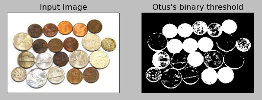
I guess the sample is tougher than the one in Image Segmentation with Watershed Algorithm because this sample has some glittering coins as well. So, unlike the OpenCV's tutorial sample, even after the Otsu's binarization, not all the coins turned into white coins.
The code looks like this:
import numpy as np
import cv2
from matplotlib import pyplot as plt

img = cv2.imread('coins.jpg')
b,g,r = cv2.split(img)
rgb_img = cv2.merge([r,g,b])

gray = cv2.cvtColor(img,cv2.COLOR_BGR2GRAY)
ret, thresh = cv2.threshold(gray,0,255,cv2.THRESH_BINARY_INV+cv2.THRESH_OTSU)

plt.subplot(121),plt.imshow(rgb_img)
plt.title('Input Image'), plt.xticks([]), plt.yticks([])
plt.subplot(122),plt.imshow(thresh, 'gray')
plt.title("Otus's binary threshold"), plt.xticks([]), plt.yticks([])
plt.show()
To remove any noise, we use morphologyEx().
# noise removal
kernel = np.ones((2,2),np.uint8)
opening = cv2.morphologyEx(thresh,cv2.MORPH_OPEN,kernel, iterations = 2)
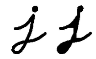
The picture below shows the effect of Opening (useful for removing small objects - it is assumed that the objects are bright on a dark foreground):
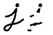
This one demonstrates the Closing Effect (useful to remove small holes - dark regions):
When I appied the Opening effect to my sample:

But in my case, the Opening does not seem to be working even with 2x2 kernel, rather it's gotten worse.
If I use Closing instead:

It seems the Closing fares better.
Here is the code:
import numpy as np
import cv2
from matplotlib import pyplot as plt

img = cv2.imread('coins.jpg')
b,g,r = cv2.split(img)
rgb_img = cv2.merge([r,g,b])

gray = cv2.cvtColor(img,cv2.COLOR_BGR2GRAY)
ret, thresh = cv2.threshold(gray,0,255,cv2.THRESH_BINARY_INV+cv2.THRESH_OTSU)

# noise removal
kernel = np.ones((2,2),np.uint8)
#opening = cv2.morphologyEx(thresh,cv2.MORPH_OPEN,kernel, iterations = 2)
closing = cv2.morphologyEx(thresh,cv2.MORPH_CLOSE,kernel, iterations = 2)

plt.subplot(131),plt.imshow(rgb_img)
plt.title('Input Image'), plt.xticks([]), plt.yticks([])
plt.subplot(132),plt.imshow(thresh, 'gray')
plt.title("Otus's binary threshold"), plt.xticks([]), plt.yticks([])
plt.subplot(133),plt.imshow(closing, 'gray')
plt.title("morphologyEx"), plt.xticks([]), plt.yticks([])
plt.show()
This operations consists of convoluting an image A with some kernel (B), which can have any shape or size, usually a square or circle.
The kernel B has a defined anchor point, usually being the center of the kernel.
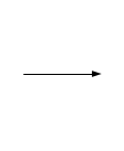
As the kernel B is scanned over the image, we compute the maximal pixel value overlapped by B and replace the image pixel in the anchor point position with that maximal value. As we can deduce, this maximizing operation causes bright regions within an image to grow. (therefore the name dilation).
Here is an example of applying the dilation operation:

# sure background area
sure_bg = cv2.dilate(closing,kernel,iterations=3)
When applied to the sample, we get:
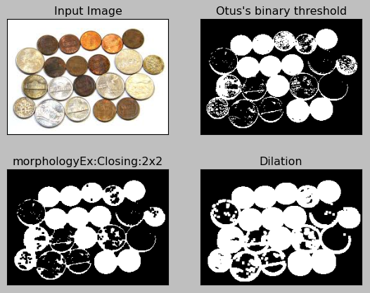
Here is the code:
import numpy as np
import cv2
from matplotlib import pyplot as plt

img = cv2.imread('coins.jpg')
b,g,r = cv2.split(img)
rgb_img = cv2.merge([r,g,b])

gray = cv2.cvtColor(img,cv2.COLOR_BGR2GRAY)
ret, thresh = cv2.threshold(gray,0,255,cv2.THRESH_BINARY_INV+cv2.THRESH_OTSU)

# noise removal
kernel = np.ones((2,2),np.uint8)
#opening = cv2.morphologyEx(thresh,cv2.MORPH_OPEN,kernel, iterations = 2)
closing = cv2.morphologyEx(thresh,cv2.MORPH_CLOSE,kernel, iterations = 2)

# sure background area
sure_bg = cv2.dilate(closing,kernel,iterations=3)

plt.subplot(221),plt.imshow(rgb_img)
plt.title('Input Image'), plt.xticks([]), plt.yticks([])
plt.subplot(222),plt.imshow(thresh, 'gray')
plt.title("Otus's binary threshold"), plt.xticks([]), plt.yticks([])
plt.subplot(223),plt.imshow(closing, 'gray')
plt.title("morphologyEx:Closing:2x2"), plt.xticks([]), plt.yticks([])
plt.subplot(224),plt.imshow(sure_bg, 'gray')
plt.title("Dilation"), plt.xticks([]), plt.yticks([])
plt.show()
Will be continued : Watershed Algorithm : Marker-based Segmentation II.
Ph.D. / Golden Gate Ave, San Francisco / Seoul National Univ / Carnegie Mellon / UC Berkeley / DevOps / Deep Learning / Visualization