Image Thresholding and Segmentation

Thresholding is the simplest method of image segmentation. It is a non-linear operation that converts a gray-scale image into a binary image where the two levels are assigned to pixels that are below or above the specified threshold value. In other words, if pixel value is greater than a threshold value, it is assigned one value (may be white), else it is assigned another value (may be black). In OpenCV, we use cv2.threshold() function:
cv2.threshold(src, thresh, maxval, type[, dst])
This function applies fixed-level thresholding to a single-channel array. The function is typically used to get a bi-level (binary) image out of a grayscale image ( compare() could be also used for this purpose) or for removing a noise, that is, filtering out pixels with too small or too large values. There are several types of thresholding supported by the function.
The function returns the computed threshold value and thresholded image.
- src - input array (single-channel, 8-bit or 32-bit floating point). This is the source image, which should be a grayscale image.
- thresh - threshold value, and it is used to classify the pixel values.
- maxval - maximum value to use with the THRESH_BINARY and THRESH_BINARY_INV thresholding types. It represents the value to be given if pixel value is more than (sometimes less than) the threshold value.
- type - thresholding type.(see threshold for details).
- cv2.THRESH_BINARY
- cv2.THRESH_BINARY_INVY
- cv2.THRESH_TRUNCY
- cv2.THRESH_TOZEROY
- cv2.THRESH_TOZERO_INVY
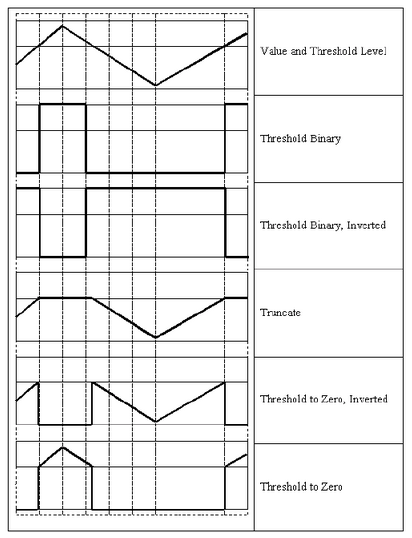
Picture source: threshold
- dst - output array of the same size and type as src.
The code looks like this:
import cv2
import numpy as np
from matplotlib import pyplot as plt

img = cv2.imread('gradient.png',0)
ret,thresh1 = cv2.threshold(img,127,255,cv2.THRESH_BINARY)
ret,thresh2 = cv2.threshold(img,127,255,cv2.THRESH_BINARY_INV)
ret,thresh3 = cv2.threshold(img,127,255,cv2.THRESH_TRUNC)
ret,thresh4 = cv2.threshold(img,127,255,cv2.THRESH_TOZERO)
ret,thresh5 = cv2.threshold(img,127,255,cv2.THRESH_TOZERO_INV)

titles = ['Original Image','BINARY','BINARY_INV','TRUNC','TOZERO','TOZERO_INV']
images = [img, thresh1, thresh2, thresh3, thresh4, thresh5]

for i in xrange(6):
    plt.subplot(2,3,i+1),plt.imshow(images[i],'gray')
    plt.title(titles[i])
    plt.xticks([]),plt.yticks([])

plt.show()
Output:
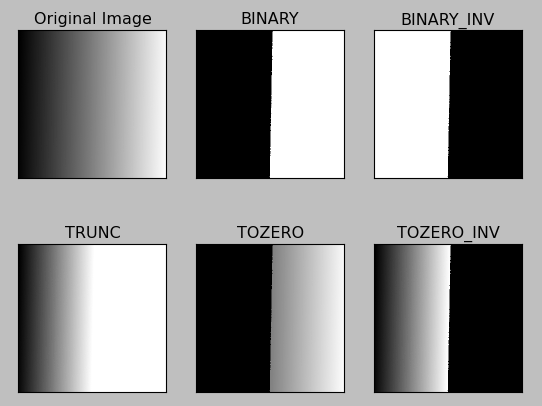
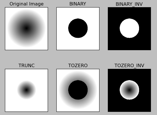
Original images are available :
gradient.png and circle.png
Using a global threshold value may not be good choicewhere image has different lighting conditions in different areas. So, in that case, we may want to use adaptive thresholding. It uses the algorithm that calculates the threshold for a small regions of the image so that we can get different thresholds for different regions of the same image and it gives us better results for images with varying light conditions.
cv.AdaptiveThreshold(src, dst, maxValue, adaptive_method=CV_ADAPTIVE_THRESH_MEAN_C, thresholdType=CV_THRESH_BINARY, blockSize=3, param1=5)
where:
- src - Source 8-bit single-channel image.
- dst - Destination image of the same size and the same type as src.
- maxValue - Non-zero value assigned to the pixels for which the condition is satisfied.
- adaptiveMethod - Adaptive thresholding algorithm to use, ADAPTIVE_THRESH_MEAN_C (hreshold value is the mean of neighbourhood area) or ADAPTIVE_THRESH_GAUSSIAN_C (threshold value is the weighted sum of neighbourhood values where weights are a gaussian window). adaptiveMethod decides how thresholding value is calculated.
- thresholdType - Thresholding type that must be either THRESH_BINARY or THRESH_BINARY_INV .
- blockSize - size of a pixel neighborhood that is used to calculate a threshold value for the pixel: 3, 5, 7, and so on.
- C - Constant subtracted from the mean or weighted mean. Normally, it is positive but may be zero or negative as well. It is just a constant which is subtracted from the mean or weighted mean calculated.
Here is the code for adaptive thresholding:
import cv2
import numpy as np
from matplotlib import pyplot as plt

img = cv2.imread('bw.png',0)
img = cv2.medianBlur(img,5)

ret,th1 = cv2.threshold(img,127,255,cv2.THRESH_BINARY)
th2 = cv2.adaptiveThreshold(img,255,cv2.ADAPTIVE_THRESH_MEAN_C,\
            cv2.THRESH_BINARY,11,2)
th3 = cv2.adaptiveThreshold(img,255,cv2.ADAPTIVE_THRESH_GAUSSIAN_C,\
            cv2.THRESH_BINARY,11,2)

titles = ['Original Image', 'Global Thresholding (v = 127)',
            'Adaptive Mean Thresholding', 'Adaptive Gaussian Thresholding']
images = [img, th1, th2, th3]

for i in xrange(4):
    plt.subplot(2,2,i+1),plt.imshow(images[i],'gray')
    plt.title(titles[i])
    plt.xticks([]),plt.yticks([])
plt.show()
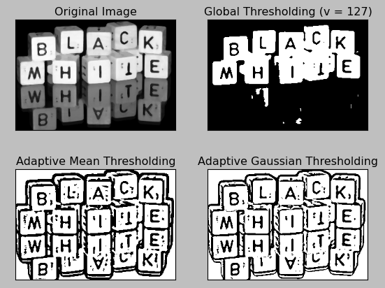
Original images :
bw.png
Otsu binarization automatically calculates a threshold value from image histogram for a bimodal image.
It uses cv2.threshold() function with an extra flag, cv2.THRESH_OTSU. For threshold value, simply pass zero. Then the algorithm finds the optimal threshold value and returns us as the second output, retVal. If Otsu thresholding is not used, the retVal remains same as the threshold value we used.
import cv2
import numpy as np
from matplotlib import pyplot as plt

img = cv2.imread('EinStein.jpg',0)

# global thresholding
ret1,th1 = cv2.threshold(img,127,255,cv2.THRESH_BINARY)

# Otsu's thresholding
ret2,th2 = cv2.threshold(img,0,255,cv2.THRESH_BINARY+cv2.THRESH_OTSU)

# Otsu's thresholding after Gaussian filtering
blur = cv2.GaussianBlur(img,(5,5),0)
ret3,th3 = cv2.threshold(blur,0,255,cv2.THRESH_BINARY+cv2.THRESH_OTSU)

# plot all the images and their histograms
images = [img, 0, th1,
          img, 0, th2,
          blur, 0, th3]
titles = ['Original Noisy Image','Histogram','Global Thresholding (v=127)',
          'Original Noisy Image','Histogram',"Otsu's Thresholding",
          'Gaussian filtered Image','Histogram',"Otsu's Thresholding"]

for i in xrange(3):
    plt.subplot(3,3,i*3+1),plt.imshow(images[i*3],'gray')
    plt.title(titles[i*3]), plt.xticks([]), plt.yticks([])
    plt.subplot(3,3,i*3+2),plt.hist(images[i*3].ravel(),256)
    plt.title(titles[i*3+1]), plt.xticks([]), plt.yticks([])
    plt.subplot(3,3,i*3+3),plt.imshow(images[i*3+2],'gray')
    plt.title(titles[i*3+2]), plt.xticks([]), plt.yticks([])
plt.show()
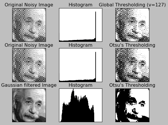
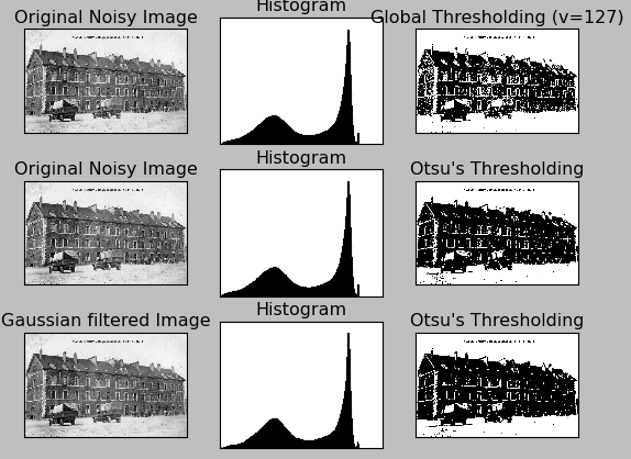
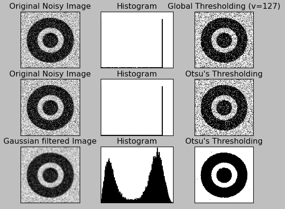
Original images :
EinStein.jpg
bimodal.jpg
bimodal_hsv_noise.png
OpenCV 3 Tutorial
image & video processing
Installing on Ubuntu 13
Mat(rix) object (Image Container)
Creating Mat objects
The core : Image - load, convert, and save
Smoothing Filters A - Average, Gaussian
Smoothing Filters B - Median, Bilateral
OpenCV 3 image and video processing with Python
OpenCV 3 with Python
Image - OpenCV BGR : Matplotlib RGB
Basic image operations - pixel access
iPython - Signal Processing with NumPy
Signal Processing with NumPy I - FFT and DFT for sine, square waves, unitpulse, and random signal
Signal Processing with NumPy II - Image Fourier Transform : FFT & DFT
Inverse Fourier Transform of an Image with low pass filter: cv2.idft()
Image Histogram
Video Capture and Switching colorspaces - RGB / HSV
Adaptive Thresholding - Otsu's clustering-based image thresholding
Edge Detection - Sobel and Laplacian Kernels
Canny Edge Detection
Hough Transform - Circles
Watershed Algorithm : Marker-based Segmentation I
Watershed Algorithm : Marker-based Segmentation II
Image noise reduction : Non-local Means denoising algorithm
Image object detection : Face detection using Haar Cascade Classifiers
Image segmentation - Foreground extraction Grabcut algorithm based on graph cuts
Image Reconstruction - Inpainting (Interpolation) - Fast Marching Methods
Video : Mean shift object tracking
Machine Learning : Clustering - K-Means clustering I
Machine Learning : Clustering - K-Means clustering II
Machine Learning : Classification - k-nearest neighbors (k-NN) algorithm
Ph.D. / Golden Gate Ave, San Francisco / Seoul National Univ / Carnegie Mellon / UC Berkeley / DevOps / Deep Learning / Visualization