Machine Learning k-nearest neighbors (k-NN) algorithm

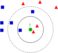
We have a new member which is shown as green circle. It should be added to one of these Blue/Red families. We call that process, classification.

"Example of k-NN classification. The test sample (green circle) should be classified either to the first class of blue squares or to the second class of red triangles. If k = 3 (solid line circle) it is assigned to the second class because there are 2 triangles and only 1 square inside the inner circle. If k = 5 (dashed line circle) it is assigned to the first class (3 squares vs. 2 triangles inside the outer circle)." - wiki - k-nearest neighbors algorithm.

This method of classification is called k-Nearest Neighbors since classification depends on k nearest neighbors.

"k-NN is a type of instance-based learning, or lazy learning, where the function is only approximated locally and all computation is deferred until classification. The k-NN algorithm is among the simplest of all machine learning algorithms."

A drawback of the basic "majority voting" classification occurs when the class distribution is skewed.

"Both for classification and regression, it can be useful to weigh the contributions of the neighbors, so that the nearer neighbors contribute more to the average than the more distant ones. For example, a common weighting scheme consists in giving each neighbor a weight of 1/d, where d is the distance to the neighbor."

The neighbors are taken from a set of objects for which the class (for k-NN classification) or the object property value (for k-NN regression) is known. This can be thought of as the training set for the algorithm, though no explicit training step is required.

"A shortcoming of the k-NN algorithm is that it is sensitive to the local structure of the data."

We will create two classes (Red and Blue), and label the Red family as Class-0 and Blue family as Class-1 with 25 training data set, and label them either Class-0 or Class-1.

We do all this using Random Number Generator in Numpy, the (x,y) coordinates will be in the range of (1, 100):

# Feature set containing (x,y) values of 25 known/training data
trainData = np.random.randint(0,100,(25,2)).astype(np.float32)

Instantiate the kNN algorithm:

knn = cv2.KNearest()

Then, we pass the trainData and responses to train the kNN:

knn.train(trainData,responses)

It will construct a search tree.

The sample should be a floating point array. The size of the sample is (# of samples) x (# of features) = (1 x 2). In other words, we will use 1 sample for two classes (Red or Blue feature), which makes the size of the same (1,2) as shown in the code:

newcomer = np.random.randint(0,100,(1,2)).astype(np.float32)

Then we find three neighbors and predicts responses for input vectors:

ret, results, neighbours ,dist = knn.find_nearest(newcomer, 3)

Actually, the syntax for find_nearest() looks like this:

cv2.KNearest.find_nearest(samples, k[, results[, neighborResponses[, dists]]]) → retval, results, neighborResponses, dists

Where the parameters are:

1. samples : Input samples stored by rows. It is a single-precision floating-point matrix of $number\_of\_samples \times number\_of\_features$ size.
2. k : Number of used nearest neighbors. It must satisfy constraint: $k \le CvKNearest::get\_max\_k()$.
3. results : Vector with results of prediction (regression or classification) for each input sample. It is a single-precision floating-point vector with number_of_samples elements.
4. neighbors : Optional output pointers to the neighbor vectors themselves. It is an array of $k*samples->rows$ pointers.
5. neighborResponses : Optional output values for corresponding neighbors. It is a single-precision floating-point matrix of $number\_of\_samples \times k$ size.
6. dist : Optional output distances from the input vectors to the corresponding neighbors. It is a single-precision floating-point matrix of $number\_of\_samples \times k$ size.

import cv2
import numpy as np
import matplotlib.pyplot as plt

# Feature set containing (x,y) values of 25 known/training data
trainData = np.random.randint(0,100,(25,2)).astype(np.float32)

# Labels each one either Red or Blue with numbers 0 and 1
responses = np.random.randint(0,2,(25,1)).astype(np.float32)

# plot Reds
red = trainData[responses.ravel()==0]
plt.scatter(red[:,0],red[:,1],80,'r','^')

# plot Blues
blue = trainData[responses.ravel()==1]
plt.scatter(blue[:,0],blue[:,1],80,'b','s')

# CvKNearest instance
knn = cv2.KNearest()

# trains the model
knn.train(trainData,responses)

# New sample : (x,y)
newcomer = np.random.randint(0,100,(1,2)).astype(np.float32)
plt.scatter(newcomer[:,0],newcomer[:,1],80,'g','o')

# Finds the 3nearest  neighbors and predicts responses for input vectors
ret, results, neighbours, dist = knn.find_nearest(newcomer, 3)

print "result: ", results,"\n"
print "neighbours: ", neighbours,"\n"
print "distance: ", dist

plt.show()  

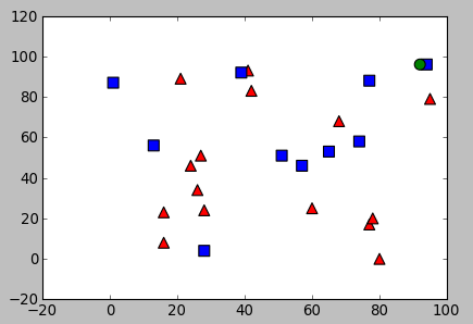
With the output:

result:  [[ 1.]] 
neighbours:  [[ 1.  1.  0.]] 
distance:  [[   4.  289.  298.]]

The result is 1 which indicate the new sample belongs blue class:

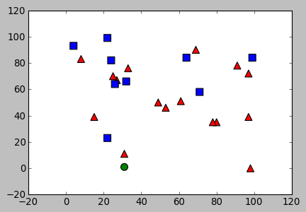
With the output:

result:  [[ 0.]] 
neighbours:  [[ 0.  1.  0.]] 
distance:  [[  100.   565.  1700.]]

The result is 0 which indicate the new sample belongs red class:

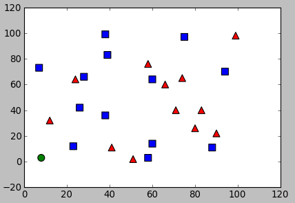
With the output:

result:  [[ 0.]] 
neighbours:  [[ 1.  0.  0.]] 
distance:  [[  306.   857.  1153.]]

The result is 0 which indicate the new sample belongs red class:

However, if we had used $k=5$, it could have been classified as blue.