scikit-learn : Supervised Learning, Unsupervised Learning, and Reinforcement learning

Supervised learning is concerned with learning a model from labeled data (training data) which has the correct answer. This allows us to make predictions about future or unseen data.

The picture below shows an example of supervised learning. It's collections of scattered points whose coordinates are size and weight. Supervised learning gives us not only the sample data but also correct answers, for this case, it's the colors or the values of the coin.

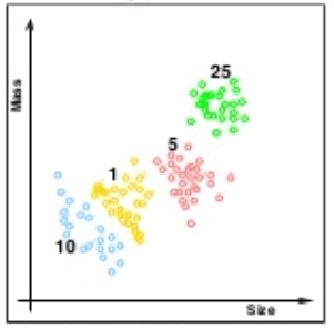
Picture source : Lecture 01 - The Learning Problem, Caltech

Regression and classification are the most common types of problems in supervised learning.

"An optimal scenario will allow for the algorithm to correctly determine the class labels for unseen instances. This requires the learning algorithm to generalize from the training data to unseen situations in a 'reasonable' way." - wiki - Supervised learning.

Unsupervised Learning's task is to construct an estimator which is able to predict the label of an object given the set of features.

Unlike the supervised learning, as we can see from the picture below, unsupervised learning does not give us the color or the value information. In other words, it only gives us sample data but not the data for correct answers:

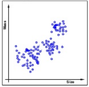
Picture source : Lecture 01 - The Learning Problem, Caltech

So, for unsupervised learning we get:

(input, ?)

instead of the following for supervised learning:

(input, correct output)

Unsupervised Learning problem is "trying to find hidden structure in unlabeled data. Since the examples given to the learner are unlabeled, there is no error or reward signal to evaluate a potential solution. This distinguishes unsupervised learning from supervised learning and reinforcement learning." - wiki - Unsupervised learning.

In supervised learning, we know the right answer beforehand when we train our model, and in reinforcement learning, we define a measure of reward for particular actions by the agent.

In unsupervised learning, however, we are dealing with unlabeled data or data of unknown structure. Using unsupervised learning techniques, we are able to explore the structure of our data to extract meaningful information without the guidance of a known outcome variable or reward function.

- Python Machine Learning by Sebastian Raschka

Simply put, the goal of unsupervised learning is to find structure in the unlabeled data. Clustering is probably the most common technique.

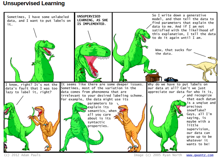
The third type of machine learning is reinforcement learning.

The goal of the reinforcement learning is to> develop a system that improves its performance based on interactions with the environment.

We could think of reinforcement learning as a supervised learning, however, in reinforcement learning the feedback (reward) from the environment is not the label or value, but a measure of how well the action was measured by the reward function.

Via the interaction with the environment, our system (agent) can then use reinforcement learning to learn a series of actions that maximizes this reward via an exploratory trial-and-error approach.

A popular example of reinforcement learning is a chess engine. Here, the agent decides upon a series of moves depending on the state of the board (the environment), and the reward can be defined as win or lose at the end of the game:

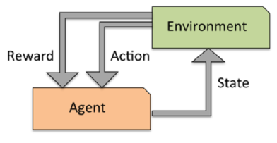
Credit: Python Machine Learning by Sebastian Raschka, 2015

The following table is Iris dataset, which is a classic example in the field of machine learning.

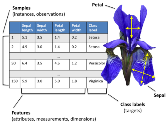
Credit: Python Machine Learning by Sebastian Raschka, 2015

Our Iris dataset contains the measurements of 150 iris flowers from three different species: Setosa, Versicolor, and Viriginica: it can then be written as a 150 x 3 matrix.

Here, each flower sample represents one row in our data set, and the flower measurements in centimeters are stored as columns, which we also call the features of the dataset.

We are given the measurements of petals and sepals. The task is to guess the class of an individual flower. It's a classification task.

>>> from sklearn.datasets import load_iris
>>> iris = load_iris()
>>> X = iris.data
>>> y = iris.target

It is trivial to train a classifier once the data has this format. A support vector machine (SVM), for instance, with a linear kernel:

>>> from sklearn.svm import LinearSVC
>>> LinearSVC()
LinearSVC(C=1.0, class_weight=None, dual=True, fit_intercept=True,
     intercept_scaling=1, loss='l2', multi_class='ovr', penalty='l2',
     random_state=None, tol=0.0001, verbose=0)
>>> clf = LinearSVC

clf is a statistical model that has hyperparameters that control the learning algorithm. Those hyperparameters can be supplied by the user in the constructor of the model.

By default the real model parameters are not initialized. The model parameters will be automatically tuned from the data by calling the fit() method:

>>> clf = clf.fit(X,y)
>>> clf.coef_
array([[ 0.18423926,  0.45122784, -0.80794282, -0.45071669],
       [ 0.04497896, -0.87929491,  0.40550806, -0.94073588],
       [-0.85087141, -0.98678139,  1.38086854,  1.8653876 ]])
>>> clf.intercept_
array([ 0.10956135,  1.67443781, -1.70981491])

Once the model is trained, it can be used to predict the most likely outcome on unseen data.

Let's try with iris.data, using the last sample:

>>> iris.data
array([[ 5.1,  3.5,  1.4,  0.2],
       [ 4.9,  3. ,  1.4,  0.2],
       [ 4.7,  3.2,  1.3,  0.2],
       ...
       [ 6.5,  3. ,  5.2,  2. ],
       [ 6.2,  3.4,  5.4,  2.3],
       [ 5.9,  3. ,  5.1,  1.8]])

>>> X_new = [[ 5.9,  3. ,  5.1,  1.8]]

>>> clf.predict(X_new)
array([2])

>>> iris.target_names
array(['setosa', 'versicolor', 'virginica'], 
      dtype='|S10')

The result is 2, and the id of the 3rd iris class, namely 'virginica'.

scikit-learn logistic regression models can further predict probabilities of the outcome.

We continue to use the data from the previous section.

>>> from sklearn.linear_model import LogisticRegression
>>> clf2 = LogisticRegression().fit(X, y)
>>> clf2
LogisticRegression(C=1.0, class_weight=None, dual=False, fit_intercept=True,
          intercept_scaling=1, penalty='l2', random_state=None, tol=0.0001)
>>> clf2.predict_proba(X_new)
array([[ 0.00168398,  0.2810578 ,  0.71725822]])

This means that the model estimates that the sample in X_new has:

1. 0.1% likelyhood to belong to the 'setosa' class
2. 28% likelyhood to belong to the 'versicolor' class
3. 71% likelyhood to belong to the 'virginica' class

Actually, the model can predict using predict() method which is based on the probability output from predict_proba():

>>> clf2.predict(X_new)
array([2])

Note: the logistic regression is not a regression method but a classification method!

When do we use logistic regression?

1. In probabilistic setups - easy to incorporate prior knowledge
2. When the number of features is pretty small - The model will tell us which features are important.
3. When the training speed is an issue - training logistic regression is relatively fast.
4. When precision is not critical.

Here we want to derive a set of new artificial features that is smaller than the original feature set while retaining most of the variance of the original data. We call this dimensionality reduction.

Principal Component Analysis (PCA) is the most common technique for dimensionality reduction. PCA does it using linear combinations of the original features through a truncated Singular Value Decomposition of the matrix X so as to project the data onto a base of the top singular vectors.

>>> from sklearn.decomposition import PCA
>>> pca = PCA(n_components=2, whiten=True).fit(X)

After the fit(), the pca model exposes the singular vectors in the components_ attribute:

>>> pca.components_
array([[ 0.17650757, -0.04015901,  0.41812992,  0.17516725],
       [-1.33840478, -1.48757227,  0.35831476,  0.15229463]])
>>> pca.explained_variance_ratio_
array([ 0.92461621,  0.05301557])
>>> pca.explained_variance_ratio_.sum() 
0.97763177502480336

Since the number of retained components is 2, we project the iris dataset along those first 2 dimensions:

>>> X_pca = pca.transform(X)

>>> import numpy as np
>>> np.round(X_pca.mean(axis=0), decimals=5)
array([-0.,  0.])
>>> np.round(X_pca.std(axis=0), decimals=5)
array([ 1.,  1.])

Also note that the samples components do no longer carry any linear correlation:

>>> import numpy as np
>>> np.round(np.corrcoef(X_pca.T), decimals=5)
array([[ 1., -0.],
       [-0.,  1.]])

Now, we can visualize the dataset using pylab, for instance by defining the utility function:

Here is the code: pca_reduction.py

from sklearn.datasets import load_iris
import pylab as pl
from itertools import cycle
from sklearn.decomposition import PCA

class pca_reduction:
	def __init__(self):
		iris = load_iris()
		self.X = iris.data
		self.y = iris.target
		self.names = iris.target_names
		self.plot()

	def plot(self):
		pca = PCA(n_components=2, whiten=True).fit(self.X)
		X_pca = pca.transform(self.X)
		plot_2D(X_pca, self.y, self.names)

def plot_2D(data, target, target_names):
	colors = cycle('rgbcmykw')
	target_ids = range(len(target_names))
	pl.figure()
	for i, c, label in zip(target_ids, colors, target_names):
		pl.scatter(data[target == i, 0], data[target == i, 1],
					c=c, label=label)
	pl.legend()
	pl.show()

if __name__ == '__main__':
	pr = pca_reduction()
	print 'X = %s' %pr.X
	print 'y = %s' %pr.y
	print 'names = %s' %pr.names

The code draws the following picture:

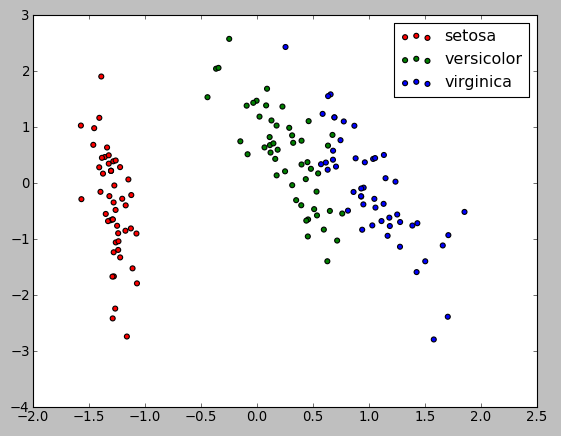
The projection was determined without any help from the labels (represented by the colors), which means this learning is unsupervised. Nevertheless, we see that the projection gives us insight into the distribution of the different flowers in parameter space: notably, iris setosa is much more distinct than the other two species as shown in the picture below:

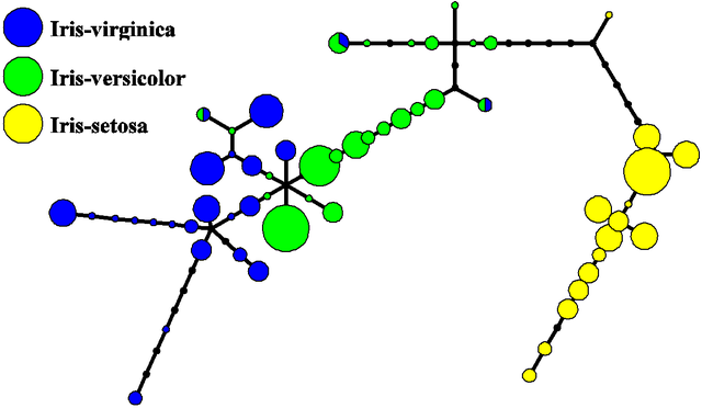
Picture source - Iris flower data set.

Machine Learning with scikit-learn

Machine learning algorithms and concepts

Artificial Neural Networks (ANN)