scikit-learn : Features and feature extraction

Machine Learning 101: General Concepts summarized Machine learning as follows:

1. Know how to extract features from real-world data in order to perform machine learning tasks.

   Feature extraction involves reducing the amount of resources required to describe a large set of data.
   When performing analysis of complex data one of the major problems stems from the number of variables involved.
   Analysis with a large number of variables generally requires a large amount of memory and computation power, also it may cause a classification algorithm to overfit to training samples and generalize poorly to new samples.
   Feature extraction is a general term for methods of constructing combinations of the variables to get around these problems while still describing the data with sufficient accuracy.
   - Feature extraction - wiki

2. Know the basic categories of supervised learning, including classification and regression problems.
3. Know the basic categories of unsupervised learning, including dimensionality reduction and clustering.
4. Understand the distinction between linearly separable and non-linearly separable data.

"Machine Learning is about building programs with tunable parameters (typically an array of floating point values) that are adjusted automatically so as to improve their behavior by adapting to previously seen data."

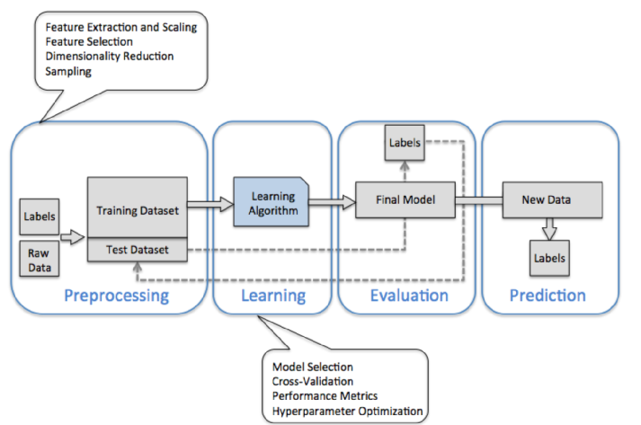
The diagram shown below is a typical workflow diagram for using machine learning.

1. Preprocessing - getting data into shape

   Raw data rarely comes in the form and shape that is necessary for the optimal performance of a learning algorithm.

   So, the preprocessing of the data is one of the most crucial steps in any machine learning application. If we take the Iris flower data set in the next section, we could think of the raw data as a series of flower images from which we want to extract meaningful features.

   Useful features could be the color, the hue, the intensity of the flowers, the height, and the flower lengths and widths.

   Some of the selected features may be highly correlated and therefore redundant to a certain degree. In those cases, dimensionality reduction techniques are useful for compressing the features onto a lower dimensional subspace. Reducing the dimensionality of our feature space has the advantage that less storage space is required, and the learning algorithm can run much faster.

2. Training and selecting a predictive model
3. Evaluating models and predicting unseen data instances

   After we have selected a model that has been fitted on the training data set, we can use the test data set to estimate how well it performs on this unseen data to estimate the generalization error.

   If we are satisfied with its performance, we can now use this model to predict new, future data.

   It is important to note that the parameters for the previously mentioned procedures such as feature scaling and dimensionality reduction are solely obtained from the training data set, and the same parameters are later reapplied to transform the test data set, as well as any new data samples.

The picture and the description of the process are from "Python Machine Learning by Sebastian Raschka, 2015"

The version numbers of the major Python packages that were used throughout this tutorial are listed below:

1. NumPy 1.9.1
2. SciPy 0.14.0
3. scikit-learn 0.15.2
4. matplotlib 1.4.0
5. pandas 0.15.2

The scikit-learn API combines a user-friendly interface with a highly optimized implementation of several classification algorithms.

The scikit-learn library offers not only a large variety of learning algorithms, but also many convenient functions such as preprocessing data, fine-tuning, and evaluating our models.

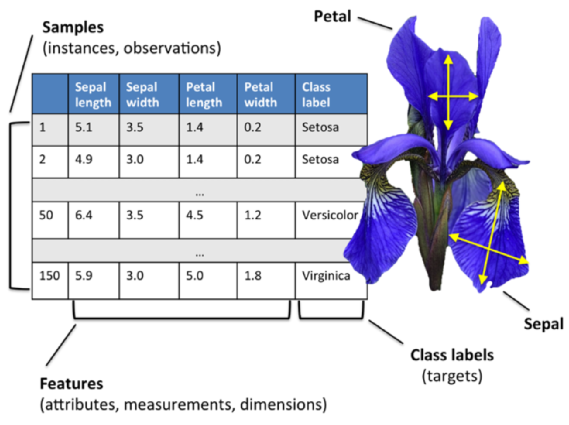
Most machine learning algorithms implemented in scikit-learn expect a numpy array as input X that has (n_samples, n_features) shape.

1. n_samples: The number of samples.
2. n_features: The number of features or distinct traits that can be used to describe each item in a quantitative manner.

Picture credit: Python Machine Learning by Sebastian Raschka, 2015

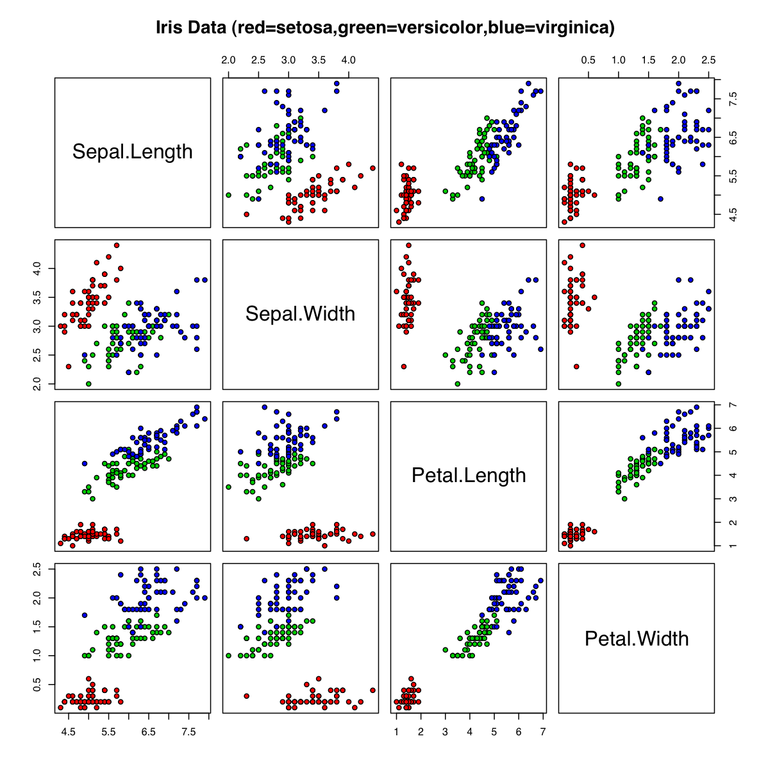
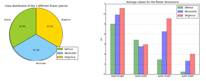
The data set of this tutorial consists of 50 samples from each of three species of Iris (Iris setosa, Iris virginica and Iris versicolor).

Four features were measured from each sample: the length and the width of the sepals and petals, in centimeters. Based on the combination of these four features, Fisher developed a linear discriminant model to distinguish the species from each other." - Iris flower data set

Picture source - Iris flower data set

Picture source - Predictive modeling, supervised machine learning, and pattern classification

scikit-learn loads data from CSV file into numpy arrays:

>>> from sklearn.datasets import load_iris
>>> iris = load_iris()

The data attribute of the dataset stores the features of each sample flower:

>>> iris.data
array([[ 5.1,  3.5,  1.4,  0.2],
       [ 4.9,  3. ,  1.4,  0.2],
       [ 4.7,  3.2,  1.3,  0.2],
       ...
       [ 6.5,  3. ,  5.2,  2. ],
       [ 6.2,  3.4,  5.4,  2.3],
       [ 5.9,  3. ,  5.1,  1.8]])
>>>
>>> n_samples, n_features = iris.data.shape
>>> n_samples
150
>>> n_features
4
>>> iris.data.shape
(150, 4)

The target attribute of the dataset stores the information about the class of each sample:

>>> len(iris.target)
150
>>> iris.target
array([0, 0, 0, 0, 0, 0, 0, 0, 0, 0, 0, 0, 0, 0, 0, 0, 0, 0, 0, 0, 0, 0, 0,
       0, 0, 0, 0, 0, 0, 0, 0, 0, 0, 0, 0, 0, 0, 0, 0, 0, 0, 0, 0, 0, 0, 0,
       0, 0, 0, 0, 1, 1, 1, 1, 1, 1, 1, 1, 1, 1, 1, 1, 1, 1, 1, 1, 1, 1, 1,
       1, 1, 1, 1, 1, 1, 1, 1, 1, 1, 1, 1, 1, 1, 1, 1, 1, 1, 1, 1, 1, 1, 1,
       1, 1, 1, 1, 1, 1, 1, 1, 2, 2, 2, 2, 2, 2, 2, 2, 2, 2, 2, 2, 2, 2, 2,
       2, 2, 2, 2, 2, 2, 2, 2, 2, 2, 2, 2, 2, 2, 2, 2, 2, 2, 2, 2, 2, 2, 2,
       2, 2, 2, 2, 2, 2, 2, 2, 2, 2, 2, 2])

The target_names attribute stores the names of the classes:

>>> iris.target_names
array(['setosa', 'versicolor', 'virginica'], 
      dtype='|S10')

If we just want a portion of dataset, for example, "Petal length" and "Petal width", we can extract like this:

>>> from sklearn import datasets
>>> import numpy as np
>>> iris = datasets.load_iris()
>>> X = iris.data[:, [2, 3]]
>>> X
array([[ 1.4,  0.2],
       [ 1.4,  0.2],
       [ 1.3,  0.2],
       [ 1.5,  0.2],
...
       [ 5. ,  1.9],
       [ 5.2,  2. ],
       [ 5.4,  2.3],
       [ 5.1,  1.8]])

If we do np.unique(y) to return the different class labels stored in iris. target, we can see Iris flower class names, Iris-Setosa, Iris-Versicolor, and Iris-Virginica, which are stored as integers ( 0 , 1 , 2 ):

>>> y = iris.target
>>> np.unique(y)
array([0, 1, 2])

Machine Learning with scikit-learn

Machine learning algorithms and concepts

Artificial Neural Networks (ANN)