Artificial Neural Network (ANN) 8 - Deep Learning I : Image Recognition (Image uploading)
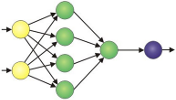
In the next couple of series of articles, we are going to learn the concepts behind multi-layer artificial neural networks.
Now that we have connected multiple neurons to a powerful neural network, we can solve complex problems such as handwritten digit recognition.
We'll use the popular back propagation algorithm, which is one of the building blocks of many neural network models that are used in deep learning, and via the back propagation algorithm, we'll be able to update the weights of such a complex neural network efficiently.
During the process, we'll make useful modifications such as mini-batch learning and an adaptive learning rate that allows us to train a neural network more efficiently.
An algorithm is considered deep if the input is passed through several non-linearities (hidden layers). Most modern learning algorithms such as decision trees, SVMs, and naive bayes are grouped as shallow.
However, in deeper network architectures, the error gradients via backpropagation would become increasingly small as more layers are added to a network. This diminishing gradient problem makes the model learning more challenging. So, special algorithms have been developed to pretrain such deep neural network structures, which is called deep learning.
In our subsequent deep learning series, we'll use one hidden layer with 50 hidden units, and will optimize approximately 1000 weights to learn a model for a very simple image classification task.
We've already covered the single-layer neural network as listed below:
1. Introduction2. Forward Propagation
3. Gradient Descent
4. Backpropagation
5. Checking gradient
6. Training via BFGS
7. Overfitting & Regularization
During the series of articles, we implemented an algorithm to perform binary classification, and we used a gradient descent optimization algorithm to learn the weight coefficients of the model. In every pass, we updated the weight vector $\mathbf w$ using the following update rule:
$$ \mathbf w:=\mathbf w+\Delta \mathbf w, \qquad \text{where} \Delta \mathbf w = - \eta \nabla J(\mathbf w) $$We computed the gradient based on the whole training set and updated the weights of the model by taking a step into the opposite direction of the gradient $\nabla J(\mathbf w)$.
We optimized the cost function $J(\mathbf w)$ which is multiplied the gradient by the learning rate $\eta$. The rate is chosen carefully to balance the speed of learning against the risk of overshooting the global minimum of the cost function.
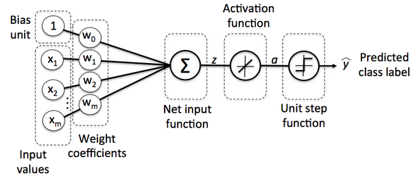
Picture source - Python Machine Learning by Sebastian Raschka
We're going to train our first multi-layer neural network to classify handwritten digits from the popular MNIST dataset (short for Mixed National Institute of Standards and Technology database) which is is publicly available at http://yann.lecun.com/exdb/mnist/:
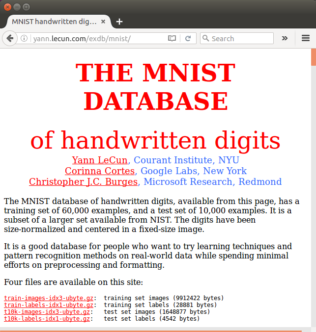
The training set consists of handwritten digits from 250 different people, 50 percent high school students, and 50 percent employees from the Census Bureau. Note that the test set contains handwritten digits from different people following the same split.
Let's download the training set images, training set labels, and unzip it:
$ wget http://yann.lecun.com/exdb/mnist/train-images-idx3-ubyte.gz
$ wget http://yann.lecun.com/exdb/mnist/train-labels-idx1-ubyte.gz
$ wget http://yann.lecun.com/exdb/mnist/t10k-images-idx3-ubyte.gz
$ wget http://yann.lecun.com/exdb/mnist/t10k-labels-idx1-ubyte.gz

$ gzip *ubyte.gz -d
Let's put the unzipped files under mnist directory.
The images are stored in byte format, and we will read them into NumPy arrays that we will use to train and test:
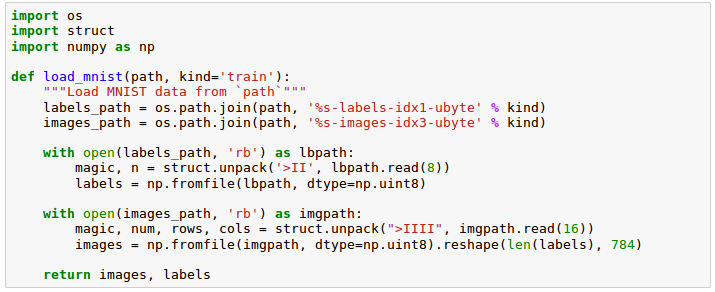
The load_mnist() function returns two arrays, the first being an $n \times m$ dimensional NumPy array (images), where $n$ is the number of samples and $m$ is the number of features.
The training dataset consists of 60,000 training digits and the test set contains 10,000 samples, respectively. The images in the MNIST dataset consist of $28 \times 28$ pixels, and each pixel is represented by a gray scale intensity value. Here, we unroll the $28 \times 28$ pixels into 1D row vectors, which represent the rows in our image array (784 per row or image).
The second array (labels) returned by the load_mnist() function contains the corresponding target variable, the class labels (integers 0-9) of the handwritten digits.
In the code, we used the following lines to read in images:
magic, n = struct.unpack('>II', lbpath.read(8))
labels = np.fromfile(lbpath, dtype=np.uint8)
Why do we need these two lines of code?
Let's take a look at the dataset file format from the MNIST website:

We first read in the magic number, which is a description of the file protocol as well as the number of items (n) from the file buffer before we read the following bytes into a NumPy array using the fromfile() method. The fmt parameter value >II that we passed as an argument to struct.unpack() has two parts:
- > : This is the big-endian. ( https://en.wikipedia.org/wiki/Endianness ).
- I : This is an unsigned integer. So, with 'II', we read in two unsigned integers.
Now we're ready to load the images. Let's do it:

We loaded 60,000 training instances and 10,000 test samples.
We may want to see what the images in MNIST look like. We can visualize examples of the digits 0-9 after reshaping the 784-pixel vectors from our feature matrix into the original $28 \times 28$ image:
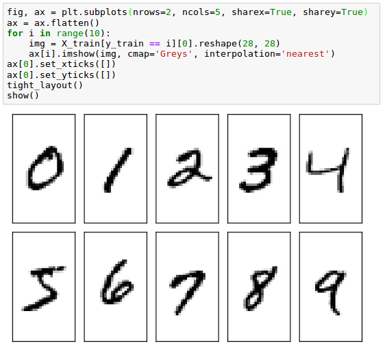
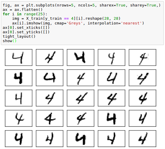
In reality, even the same digit can have numerous different hand writing:
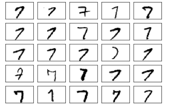
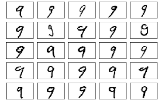
Other digits such as 7 and 9 look like the following two pictures:
Python Machine Learning by Sebastian Raschka
part8-9-ImageRecognition.ipynb
Artificial Neural Network (ANN) 9 - Deep Learning II : Image Recognition (Image classification)
Machine Learning with scikit-learn
scikit-learn installation
scikit-learn : Features and feature extraction - iris dataset
scikit-learn : Machine Learning Quick Preview
scikit-learn : Data Preprocessing I - Missing / Categorical data
scikit-learn : Data Preprocessing II - Partitioning a dataset / Feature scaling / Feature Selection / Regularization
scikit-learn : Data Preprocessing III - Dimensionality reduction vis Sequential feature selection / Assessing feature importance via random forests
Data Compression via Dimensionality Reduction I - Principal component analysis (PCA)
scikit-learn : Data Compression via Dimensionality Reduction II - Linear Discriminant Analysis (LDA)
scikit-learn : Data Compression via Dimensionality Reduction III - Nonlinear mappings via kernel principal component (KPCA) analysis
scikit-learn : Logistic Regression, Overfitting & regularization
scikit-learn : Supervised Learning & Unsupervised Learning - e.g. Unsupervised PCA dimensionality reduction with iris dataset
scikit-learn : Unsupervised_Learning - KMeans clustering with iris dataset
scikit-learn : Linearly Separable Data - Linear Model & (Gaussian) radial basis function kernel (RBF kernel)
scikit-learn : Decision Tree Learning I - Entropy, Gini, and Information Gain
scikit-learn : Decision Tree Learning II - Constructing the Decision Tree
scikit-learn : Random Decision Forests Classification
scikit-learn : Support Vector Machines (SVM)
scikit-learn : Support Vector Machines (SVM) II
Flask with Embedded Machine Learning I : Serializing with pickle and DB setup
Flask with Embedded Machine Learning II : Basic Flask App
Flask with Embedded Machine Learning III : Embedding Classifier
Flask with Embedded Machine Learning IV : Deploy
Flask with Embedded Machine Learning V : Updating the classifier
scikit-learn : Sample of a spam comment filter using SVM - classifying a good one or a bad one
Machine learning algorithms and concepts
Batch gradient descent algorithmSingle Layer Neural Network - Perceptron model on the Iris dataset using Heaviside step activation function
Batch gradient descent versus stochastic gradient descent
Single Layer Neural Network - Adaptive Linear Neuron using linear (identity) activation function with batch gradient descent method
Single Layer Neural Network : Adaptive Linear Neuron using linear (identity) activation function with stochastic gradient descent (SGD)
Logistic Regression
VC (Vapnik-Chervonenkis) Dimension and Shatter
Bias-variance tradeoff
Maximum Likelihood Estimation (MLE)
Neural Networks with backpropagation for XOR using one hidden layer
minHash
tf-idf weight
Natural Language Processing (NLP): Sentiment Analysis I (IMDb & bag-of-words)
Natural Language Processing (NLP): Sentiment Analysis II (tokenization, stemming, and stop words)
Natural Language Processing (NLP): Sentiment Analysis III (training & cross validation)
Natural Language Processing (NLP): Sentiment Analysis IV (out-of-core)
Locality-Sensitive Hashing (LSH) using Cosine Distance (Cosine Similarity)
Artificial Neural Networks (ANN)
[Note] Sources are available at Github - Jupyter notebook files1. Introduction
2. Forward Propagation
3. Gradient Descent
4. Backpropagation of Errors
5. Checking gradient
6. Training via BFGS
7. Overfitting & Regularization
8. Deep Learning I : Image Recognition (Image uploading)
9. Deep Learning II : Image Recognition (Image classification)
10 - Deep Learning III : Deep Learning III : Theano, TensorFlow, and Keras
Ph.D. / Golden Gate Ave, San Francisco / Seoul National Univ / Carnegie Mellon / UC Berkeley / DevOps / Deep Learning / Visualization