Logistic Regression

---

---

Logistic regression, in spite of its name, is a model for classification, not for regression.

Although the perceptron model is a nice introduction to machine learning algorithms for classification, its biggest disadvantage is that it never converges if the classes are not perfectly linearly separable.

Logistic regression is another simple yet more powerful algorithm for linear and binary classification problems. It is one of the most widely used algorithms for classification in industry since it is very easy to implement while performs very well on linearly separable classes.

Though it is a linear model for binary classification, it can be extended to multiclass classification as well.

To understand logistic regression as a probabilistic model, we may want to start with the odds ratio: a ratio of two odds.

Let's compare the odds ratio with probability for a case of getting "1" for dice roll:

1. Probability of getting 1 $$ p=\frac {\text {outcomes of interest}}{\text {all possible outcomes}} = 1/6$$
2. Odds for getting 1 $$ odds_{(1)} = \frac {\text {occurring}} {\text {not occurring}} = \frac {p_{(1)}} {1-p_{(1)}} = \frac {1/6} {5/6} = 1/5 = 0.2 \; or \; 1:5$$
3. Odds of getting others $$ odds_{(others)} = \frac {\text {occurring}} {\text {not occurring}} = \frac {p_{(others)}} {1-p_{(others)}} = \frac {5/6} {1/6} = \frac {5}{1} = 5 \; or \; 5:1$$
4. Odd ratio (OR) of getting 1: $$ OR_1 = \frac {odds_{(1)}} {odds_{(others)}} = \frac {1/5}{5/1} = \frac {1}{25} = 0.04 \; or \; 1:25$$
5. This tells that the odds of getting "1" on a dice roll are 1/25 less than getting others(2-6).
6. So, we got the concepts for "probability", "odds", and "odds ratio", and these are the core piece of concepts to understand/interpret the output from "logistic regression".

The power of odds ratio comes from the fact that it tells how one unit change in X affects on the predicted outcome of the model when other variables held constant.

More formally, "The odds ratio for a variable in logistic regression represents how the odds change with a 1 unit increase in that variable holding all other variables constant."

For example, let's think about the studies on diabetes with body weight.

1. We know that the weight has some effects on diabetes.
2. We have two categories: (diabetes / no diabetes).
3. Suppose, the "weight" variable has an odds ratio of 1.08.
4. This means a 1 kg increase in weight increases the odds of having diabetes by a factor of "1.08", i.e., 8%.
5. A 10 kg weight increase in increases the odds to 2.15, or more than doubles a person's odds of having diabetes, and 20 kg increases raises the odds to 4.66 or almost 5x greater.
6. One important fact we can get: the increase of the odds holds true at any weight. In other words, we have constant odds ratio. So, the increase of the odds remains the same regardless of the starting weight : 5x for 20 kg increase (no difference if it is 50->70kg or 250->270kg).
7. Another important thing to understand is that we should be able to separate probability and odds.
8. In our weight example with diabetes, people gaining 20 kg increases their odds of diabetes by 5 regardless of their starting weight.
9. However, the probability of having diabetes is lower in people with lower body weight to begin with.
10. So, even though the odds of diabetes are 5x greater with 20kg gain in body weight, the probability of having diabetes for a 50 kg person may be much lower than for a 250kg person.
11. What does it mean?
12. What that means is that the odds can have a large value even if the underlying probabilities remain low.
13. So, let's keep in mind that the odds and probability are much different when we interpret the output from the logistic regression.

The logit (loh-jit) function is the inverse of the sigmoidal "logistic" function or logistic transform used in mathematics, especially in statistics.
When the function's parameter represents a probability $p$, the logit function gives the log-odds, or the logarithm of the odds $ \frac {p}{1 - p}$.

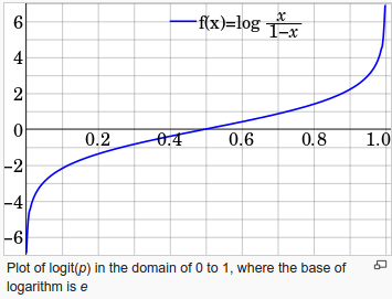
source : Logit - wiki

The logit function takes input values (probability) in the range 0 to 1 and transforms them to values over the entire real number range, which we can use to express a linear relationship between feature values and the log-odds:

$$ logit(p(y=1|x)) = \sum_{i=0}^m w_i x_i = w^Tx$$

where $p ( y = 1| x )$ is the conditional probability that a particular sample belongs to class 1 given its features $x$.

Note that the $logit(p)=log \frac{p}{1-p}$ becomes $0$ when $p=0.5$:

$$ log(.5/.5)=log(1)=0$$

So, when the probability is 0.5, in other words, odds are even, then $logit(p)=0!

Our logit function in the previous section, 0 to 1 ran along the x-axis but what we want is to have the probabilityes on the y-axis. Actually, we are interested in is predicting the probability that a certain sample belongs to a particular class.

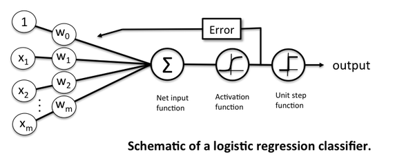
So, we want to take the inverse form of the logit function which is called the logistic function (sigmoid function):

$$ \phi(z) = \frac {1}{1+e^{-z}} = \frac {e^z}{1+e^z}$$

where $z$ is the net input which is the linear combination of variables and their coefficient. More specifically, the $z$ will be the linear combination of weights and sample features and can be expressed like this:

$$ z = w^T x = w_0 x_0 + w_1 x_1 + \;... \; + w_m x_m = w_0 + w_1 x_1 + \;...\; + w_m x_m$$

So, the inverse-logit will return the probability of being a "1" when the event occurs.

In the next section, we'll see how the inverse-logit looks like.

Let's plot the sigmoid function using matplotlib and numpy libs.

Due to the nature of the exponential function $e^{-z}$, it is often sufficient to compute the standard logistic function for x over a small range of real numbers such as a range contained in [-6, +6].

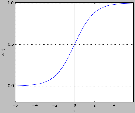
The code used for the plot:

import matplotlib.pyplot as plt
import numpy as np

def sigmoid(z):
   return 1.0 / (1.0 + np.exp(-z))

z = np.arange(-6, 6, 0.1)
phi_z = sigmoid(z)
plt.plot(z, phi_z)
plt.axvline(0.0, color='k')
plt.axhspan(0.0, 1.0, facecolor='1.0', alpha=1.0, ls='dotted')
plt.axhline(y=0.5, ls='dotted', color='k')
plt.yticks([0.0, 0.5, 1.0])
plt.ylim(-0.1, 1.1)
plt.xlabel('z')
plt.ylabel('$\phi(z)$')
plt.show()

A sigmoid function is a mathematical function having an "S" shaped curve (sigmoid curve). Often, sigmoid function refers to the special case of the logistic function shown in the figure above.

There are other sigmoid functions. In the following picture, all functions are normalized in such a way that their slope at the origin is 1.

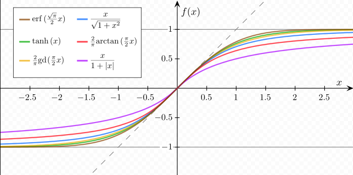
source : https://en.wikipedia.org/wiki/Sigmoid_function.

Here is a list of the most common activation functions:

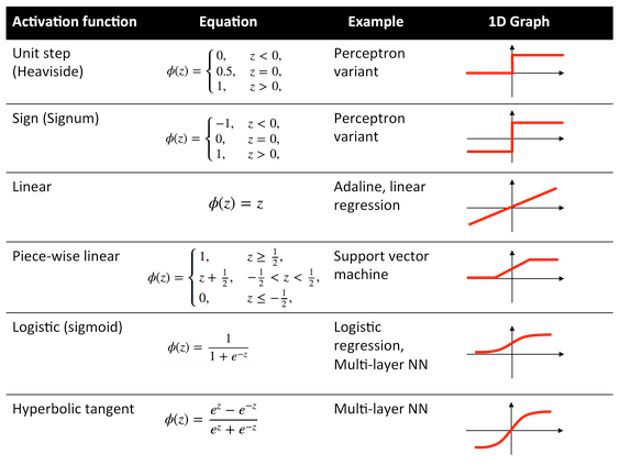
source : What is the role of the activation function in a neural network?.

"The logistic regression classifier has a non-linear activation function, but the weight coefficients of this model are essentially a linear combination, which is why logistic regression is a "generalized" linear model."

The output of the sigmoid function is interpreted as the probability of particular sample belonging to class 1, $\phi(z) = p ( y = 1| x ; w )$, given its features $x$ parameterized by the weights $w$.

For example, if we get $\phi(z) = 0.8$ for a particular flower sample, it means that the chance that this sample is an Iris-Versicolor flower is 80 percent.

Similarly, the probability that this flower is an Iris-Setosa flower can be calculated as $p( y = 0 | x ; w ) = 1 - p ( y = 1| x ; w )=0.2$ or 20 %.

The predicted probability can then simply be converted into a binary outcome via a quantizer (unit step function):

$$\hat y = \begin{cases}1 & if \; \phi(z) \ge 0.5 \\ 0 & \text{otherwise} \end{cases}$$

With sigmoid function, this is equivalent to the following:

$$\hat y = \begin{cases}1 & if \; z \ge 0.5 \\ 0 & \text{otherwise} \end{cases}$$

In fact, there are many applications where we are not only interested in the predicted class labels, but also interested in estimating the class-membership probability.

In weather forecasting, for example, logistic regression is used not only to predict if it will rain but also to report the chance of rain.

That's one of the reasons why logistic regression enjoys wide popularity in the field of medicine since logistic regression can be used to predict the chance that a patient has a particular disease given certain symptoms.

This tutorial is largely based on "Python Machine Learning: Sebastian Raschka".

Machine Learning with scikit-learn

scikit-learn installation

scikit-learn : Features and feature extraction - iris dataset

scikit-learn : Machine Learning Quick Preview

scikit-learn : Data Preprocessing I - Missing / Categorical data

scikit-learn : Data Preprocessing II - Partitioning a dataset / Feature scaling / Feature Selection / Regularization

scikit-learn : Data Preprocessing III - Dimensionality reduction vis Sequential feature selection / Assessing feature importance via random forests

Data Compression via Dimensionality Reduction I - Principal component analysis (PCA)

scikit-learn : Data Compression via Dimensionality Reduction II - Linear Discriminant Analysis (LDA)

scikit-learn : Data Compression via Dimensionality Reduction III - Nonlinear mappings via kernel principal component (KPCA) analysis

scikit-learn : Logistic Regression, Overfitting & regularization

scikit-learn : Supervised Learning & Unsupervised Learning - e.g. Unsupervised PCA dimensionality reduction with iris dataset

scikit-learn : Unsupervised_Learning - KMeans clustering with iris dataset

scikit-learn : Linearly Separable Data - Linear Model & (Gaussian) radial basis function kernel (RBF kernel)

scikit-learn : Decision Tree Learning I - Entropy, Gini, and Information Gain

scikit-learn : Decision Tree Learning II - Constructing the Decision Tree

scikit-learn : Random Decision Forests Classification

scikit-learn : Support Vector Machines (SVM)

scikit-learn : Support Vector Machines (SVM) II

Flask with Embedded Machine Learning I : Serializing with pickle and DB setup

Flask with Embedded Machine Learning II : Basic Flask App

Flask with Embedded Machine Learning III : Embedding Classifier

Flask with Embedded Machine Learning IV : Deploy

Flask with Embedded Machine Learning V : Updating the classifier

scikit-learn : Sample of a spam comment filter using SVM - classifying a good one or a bad one

---

Machine learning algorithms and concepts

Batch gradient descent algorithm

Single Layer Neural Network - Perceptron model on the Iris dataset using Heaviside step activation function

Batch gradient descent versus stochastic gradient descent

Single Layer Neural Network - Adaptive Linear Neuron using linear (identity) activation function with batch gradient descent method

Single Layer Neural Network : Adaptive Linear Neuron using linear (identity) activation function with stochastic gradient descent (SGD)

Logistic Regression

VC (Vapnik-Chervonenkis) Dimension and Shatter

Bias-variance tradeoff

Maximum Likelihood Estimation (MLE)

Neural Networks with backpropagation for XOR using one hidden layer

minHash

tf-idf weight

Natural Language Processing (NLP): Sentiment Analysis I (IMDb & bag-of-words)

Natural Language Processing (NLP): Sentiment Analysis II (tokenization, stemming, and stop words)

Natural Language Processing (NLP): Sentiment Analysis III (training & cross validation)

Natural Language Processing (NLP): Sentiment Analysis IV (out-of-core)

Locality-Sensitive Hashing (LSH) using Cosine Distance (Cosine Similarity)

---

Artificial Neural Networks (ANN)

[Note] Sources are available at Github - Jupyter notebook files

1. Introduction

2. Forward Propagation

3. Gradient Descent

4. Backpropagation of Errors

5. Checking gradient

6. Training via BFGS

7. Overfitting & Regularization

8. Deep Learning I : Image Recognition (Image uploading)

9. Deep Learning II : Image Recognition (Image classification)

10 - Deep Learning III : Deep Learning III : Theano, TensorFlow, and Keras