scikit-learn : Machine Learning Quick Preview

We can easily get Iris dataset via scikit-learn.
Since the dataset is a simple while it is the most popular dataset frequently used for testing and experimenting with algorithms, we will use it in this tutorial.
But we will only use two features from the Iris flower dataset.
We will train a perceptron model implemented in:
- Single Layer Neural Network - Perceptron model on the Iris dataset using Heaviside step activation function
- Single Layer Neural Network - Adaptive Linear Neuron using linear (identity) activation function with batch gradient descent method
- Single Layer Neural Network : Adaptive Linear Neuron using linear (identity) activation function with stochastic gradient descent (SGD)
The data set consists of 50 samples from each of three species of Iris (Iris setosa, Iris virginica and Iris versicolor). Four features were measured from each sample: the length and the width of the sepals and petals, in centimeters.
However, we will only use two features from the Iris flower dataset in this section.
from sklearn import datasets
import numpy as np
iris = datasets.load_iris()
>>> X = iris.data[:,[2,3]]
>>> y = iris.target
To evaluate how well a trained model is performing on unseen data, we will further split the dataset into separate training and test datasets:
>>> from sklearn.cross_validation import train_test_split
>>> X_train, X_test, y_train, y_test = train_test_split(X, y, test_size=0.3, random_state=0)
In the code above, we randomly split the X and y arrays into 30 percent test data (45 samples) and 70 percent training data (105 samples).
We also want to do feature scaling for optimal performance of our algorithm using the StandardScaler class from scikit-learn's preprocessing module:
>>> from sklearn.preprocessing import StandardScaler
>>> sc = StandardScaler()
>>> sc.fit(X_train)
>>> X_train_std = sc.transform(X_train)
>>> X_test_std = sc.transform(X_test)
As we can see from the code, we initialized a new StandardScaler object.
Using the fit method, StandardScaler estimated the parameters $\mu$ (sample mean) and $\sigma$ (standard deviation) for each feature dimension from the training data.
By calling the transform method, we then standardized the training data using those estimated parameters $\mu$ and $\sigma$.
Here we used the same scaling parameters to standardize the test set so that both the values in the training and test dataset are comparable to each other.
Now that we have standardized the training data, we can train a perceptron model.
Most of the algorithms in scikit-learn support multiclass classification by default via the One-vs.-Rest (OvR) method. It allows us to feed the three flower classes to the perceptron all at once.
The code looks like the following:
>>> from sklearn.linear_model import Perceptron
>>> ppn = Perceptron(n_iter=40, eta0=0.1, random_state=0)
>>> ppn.fit(X_train_std, y_train)
After loading the Perceptron class from the linear_model module, we initialized a new Perceptron object and trained the model via the fit method.
Here, the model parameter eta0 is the learning rate $\eta$.
To find an proper learning rate requires some experimentation.
If the learning rate is too large, the algorithm will overshoot the global cost minimum while if the learning rate is too small, the algorithm requires more epochs until convergence, which can make the learning slow, especially for large datasets.
Also, we used the random_state parameter for reproducibility of the initial shuffling of the training dataset after each epoch.
Now that we've trained a model in scikit-learn, we can make predictions via the predict method.
>>> y_pred = ppn.predict(X_test_std)
>>> print('Misclassified samples: %d' % (y_test != y_pred).sum())
Misclassified samples: 18
Here, y_test are the true class labels and y_pred are the class labels that we predicted.
We see that the perceptron misclassifies 18 out of the 45 flower samples. Thus, the misclassification error on the test dataset is 0.4 or 40 percent ( 18 / 45 ~ 0.4 ).
Scikit-learn also implements a large variety of different performance metrics that are available via the metrics module.
For example, we can calculate the classification accuracy of the perceptron on the test set as follows:
>>> from sklearn.metrics import accuracy_score
>>> print('Accuracy: %.2f' % accuracy_score(y_test, y_pred))
Accuracy: 0.60
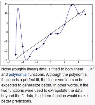
Let's learn a terminology of machine learning: overfitting.
In statistics and machine learning, one of the most common tasks is to fit a "model" to a set of training data, so as to be able to make reliable predictions on general untrained data.
In overfitting, a statistical model describes random error or noise instead of the underlying relationship.
Overfitting occurs when a model is excessively complex, such as having too many parameters relative to the number of observations.
A model that has been overfit has poor predictive performance, as it overreacts to minor fluctuations in the training data.

From Overfitting - wiki
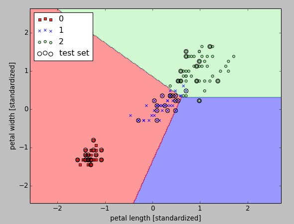
Now, we want to plot decisionregions of our trained perceptron model and visualize how well it separates the different flower samples.
from matplotlib.colors import ListedColormap
import matplotlib.pyplot as plt

def plot_decision_regions(X, y, classifier, test_idx=None, resolution=0.02):
   # setup marker generator and color map
   markers = ('s', 'x', 'o', '^', 'v')
   colors = ('red', 'blue', 'lightgreen', 'gray', 'cyan')
   cmap = ListedColormap(colors[:len(np.unique(y))])

   # plot the decision surface
   x1_min, x1_max = X[:, 0].min() - 1, X[:, 0].max() + 1
   x2_min, x2_max = X[:, 1].min() - 1, X[:, 1].max() + 1
   xx1, xx2 = np.meshgrid(np.arange(x1_min, x1_max, resolution),
   np.arange(x2_min, x2_max, resolution))
   Z = classifier.predict(np.array([xx1.ravel(), xx2.ravel()]).T)
   Z = Z.reshape(xx1.shape)
   plt.contourf(xx1, xx2, Z, alpha=0.4, cmap=cmap)
   plt.xlim(xx1.min(), xx1.max())
   plt.ylim(xx2.min(), xx2.max())

   # plot all samples
   X_test, y_test = X[test_idx, :], y[test_idx]
   for idx, cl in enumerate(np.unique(y)):
      plt.scatter(x=X[y == cl, 0], y=X[y == cl, 1],
               alpha=0.8, c=cmap(idx),
               marker=markers[idx], label=cl)
   # highlight test samples
   if test_idx:
      X_test, y_test = X[test_idx, :], y[test_idx]
      plt.scatter(X_test[:, 0], X_test[:, 1], c='',
               alpha=1.0, linewidth=1, marker='o',
               s=55, label='test set')

X_combined_std = np.vstack((X_train_std, X_test_std))
y_combined = np.hstack((y_train, y_test))
plot_decision_regions(X=X_combined_std, y=y_combined,
                      classifier=ppn, test_idx=range(105,150))
plt.xlabel('petal length [standardized]')
plt.ylabel('petal width [standardized]')
plt.legend(loc='upper left')
plt.show()
Here is result from the run.

The perceptron algorithm never converges on datasets that aren't perfectly linearly separable, which is why the use of the perceptron algorithm is typically not recommended in practice.
Later, we will look at more powerful linear classifiers that converge to a cost minimum even if the classes are not perfectly linearly separable.
This tutorial is largely based on "Python Machine Learning" by Sebastian Raschka
Machine Learning with scikit-learn
scikit-learn installation
scikit-learn : Features and feature extraction - iris dataset
scikit-learn : Machine Learning Quick Preview
scikit-learn : Data Preprocessing I - Missing / Categorical data
scikit-learn : Data Preprocessing II - Partitioning a dataset / Feature scaling / Feature Selection / Regularization
scikit-learn : Data Preprocessing III - Dimensionality reduction vis Sequential feature selection / Assessing feature importance via random forests
Data Compression via Dimensionality Reduction I - Principal component analysis (PCA)
scikit-learn : Data Compression via Dimensionality Reduction II - Linear Discriminant Analysis (LDA)
scikit-learn : Data Compression via Dimensionality Reduction III - Nonlinear mappings via kernel principal component (KPCA) analysis
scikit-learn : Logistic Regression, Overfitting & regularization
scikit-learn : Supervised Learning & Unsupervised Learning - e.g. Unsupervised PCA dimensionality reduction with iris dataset
scikit-learn : Unsupervised_Learning - KMeans clustering with iris dataset
scikit-learn : Linearly Separable Data - Linear Model & (Gaussian) radial basis function kernel (RBF kernel)
scikit-learn : Decision Tree Learning I - Entropy, Gini, and Information Gain
scikit-learn : Decision Tree Learning II - Constructing the Decision Tree
scikit-learn : Random Decision Forests Classification
scikit-learn : Support Vector Machines (SVM)
scikit-learn : Support Vector Machines (SVM) II
Flask with Embedded Machine Learning I : Serializing with pickle and DB setup
Flask with Embedded Machine Learning II : Basic Flask App
Flask with Embedded Machine Learning III : Embedding Classifier
Flask with Embedded Machine Learning IV : Deploy
Flask with Embedded Machine Learning V : Updating the classifier
scikit-learn : Sample of a spam comment filter using SVM - classifying a good one or a bad one
Machine learning algorithms and concepts
Batch gradient descent algorithmSingle Layer Neural Network - Perceptron model on the Iris dataset using Heaviside step activation function
Batch gradient descent versus stochastic gradient descent
Single Layer Neural Network - Adaptive Linear Neuron using linear (identity) activation function with batch gradient descent method
Single Layer Neural Network : Adaptive Linear Neuron using linear (identity) activation function with stochastic gradient descent (SGD)
Logistic Regression
VC (Vapnik-Chervonenkis) Dimension and Shatter
Bias-variance tradeoff
Maximum Likelihood Estimation (MLE)
Neural Networks with backpropagation for XOR using one hidden layer
minHash
tf-idf weight
Natural Language Processing (NLP): Sentiment Analysis I (IMDb & bag-of-words)
Natural Language Processing (NLP): Sentiment Analysis II (tokenization, stemming, and stop words)
Natural Language Processing (NLP): Sentiment Analysis III (training & cross validation)
Natural Language Processing (NLP): Sentiment Analysis IV (out-of-core)
Locality-Sensitive Hashing (LSH) using Cosine Distance (Cosine Similarity)
Artificial Neural Networks (ANN)
[Note] Sources are available at Github - Jupyter notebook files1. Introduction
2. Forward Propagation
3. Gradient Descent
4. Backpropagation of Errors
5. Checking gradient
6. Training via BFGS
7. Overfitting & Regularization
8. Deep Learning I : Image Recognition (Image uploading)
9. Deep Learning II : Image Recognition (Image classification)
10 - Deep Learning III : Deep Learning III : Theano, TensorFlow, and Keras
Ph.D. / Golden Gate Ave, San Francisco / Seoul National Univ / Carnegie Mellon / UC Berkeley / DevOps / Deep Learning / Visualization