Logistic Regression, Overfitting & regularization

Logistic regression is a generalized linear model using the same underlying formula, but instead of the continuous output, it is regressing for the probability of a categorical outcome.
In other words, it deals with one outcome variable with two states of the variable - either 0 or 1.
The following picture compares the logistic regression with other linear models:

Here are the sample cases with 3 linear models related to the credit analysis:

picture source: Caltech : Lecture 09 - The Linear Model II
The signal $s$ in the figure is defined as the following:
$$ s = \sum_{i=0}^n w_i x_i = \mathbf w^T \mathbf x$$Note that the linear regression does nothing to the signal while logistic regression processes the signal via the added non-linear probability ($\theta$), and the output from the logistic regression is interpreted as the probability.
For example, we can think of the $\theta(s)$ as the "probability of a heart attack" and the signal $s$ as a "risk factor".
Usually, the logistic function is given like this (sigmoid):
$$ \theta (s) = \frac {e^s}{1+e^s} $$The likelihood for a given data $(x,y)$ becomes:
$$ P(y|\mathbf x) = \theta(y\mathbf w^T \mathbf x)$$For a given whole data set, the likelihood should be like this:
$$ \prod_{n=1}^N \theta(y_n \color{purple}{\mathbf w}^T \mathbf x_n)$$Now we want to maximize with respect to our parameter $\color{purple}{w}$ which in turn to a problem of minimizing the "in sample error" that can be defined as following:
$$ E_{in}(\color{purple}{\mathbf w}) = \frac {1}{N} \sum_{n=1}^N \ln \left( \frac{1}{\theta(y_n \color{purple}{\mathbf w}^T \mathbf x_n)} \right) $$If we use the sigmoid, the in-sample error for logistic regression becomes:
$$ E_{in}(\color{purple}{\mathbf w}) = \frac {1}{N} \sum_{n=1}^N \underbrace{ \ln \left( 1 + e^{-y_n \color{purple}{\mathbf w}^T \mathbf x_n} \right) }_{\text{ "cross-entropy" error}}$$At this point, we can compare it with the one for linear regression:
$$ E_{in}(\color{purple}{\mathbf w}) = \frac {1}{N} \sum_{n=1}^N \left( \color{purple}{\mathbf w}^T \mathbf x_n - y_n \right)^2$$To minimize the error we use the general method for nonlinear optimization called gradient descent method.
The $\Delta E_{in}$ can be calculated as the following:
$$ \Delta E_{in} \ge \eta \Vert {\nabla E_{in} \left( \mathbf w(0) \right)} \Vert$$where $\eta$ is the stp size.
So, the steepest univ vector ($\hat n$) can be given as:
$$ \hat n = - \frac {\nabla E_{in} \left( \mathbf w(0) \right)} { \Vert {\nabla E_{in} \left( \mathbf w(0) \right)} \Vert } $$$ \Delta \mathbf w$ becomes:
$$ \Delta \mathbf w = -\eta \frac {\nabla E_{in} \left( \mathbf w(0) \right)} { \Vert {\nabla E_{in} \left( \mathbf w(0) \right)} \Vert } $$If we use learning rate ($\eta_{learn}$):
$$ \Delta \mathbf w = -\eta_{learn} \nabla E_{in} \left( \mathbf w(0) \right) $$So, in each iteration, the weight($w$) can be updated like this:
$$ w(t+1) = w(t)-\eta_{learn} \nabla E_{in}$$where $\nabla E_{in}$ is:
$$ \nabla E_{in} = \frac{1}{N} \sum_{n=1}^N \frac {y_n \mathbf x_n}{1+e^{y_n \mathbf w^T \mathbf x_n}}$$In Maximum Likelihood Estimation (MLE), we get the following cost function:
$$ J(w) = \sum_i^n -y^{(i)}log(\phi(z^{(i)})-(1-y^{(i)})log(1-\phi(z^{(i)}))$$We can implement the cost function for our own logistic regression.
The scikit-learn, however, implements a highly optimized version of logistic regression that also supports multiclass settings off-the-shelf, we will skip our own implementation and use the sklearn.linear_model.LogisticRegression class instead.
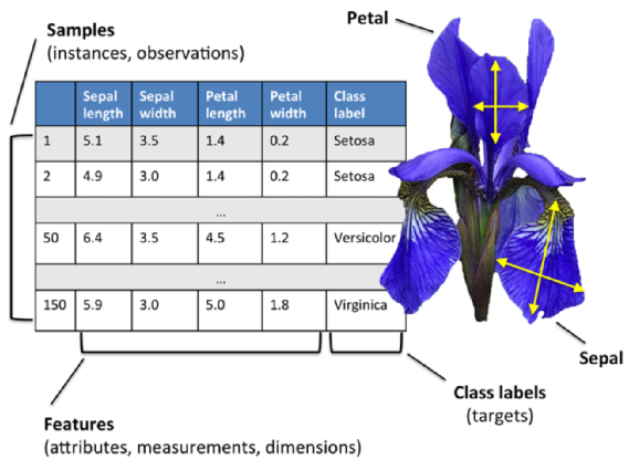
For the iris-dataset, as we've done before, we splited the set into separate training and test datasets: we randomly split the X and y arrays into 30 percent test data(45 samples, index 105-149) and 70 percent training data(105, index 0-104) samples.
We also did feature scaling for optimal performance of our algorithm suing the StandardScaler class from scikit-learn's preprocessing module.
Also, by using the fit method, StandardScaler estimated the parameter $\mu$ (sample mean) and $\sigma$ (standard deviation) for each feature dimension from the training data.
Then, by calling the transform method, we standardized the training data using those $\mu$ and $\sigma$.
For the testing data, we used the same scaling parameters to standardize the set so that both the values in the training and test dataset are comparable to each other.
Here is the code for the scikit-learn's logistic regression:
# scikit-learn logistic regression

from sklearn import datasets
import numpy as np
iris = datasets.load_iris()
X = iris.data[:, [2, 3]]
y = iris.target

from sklearn.cross_validation import train_test_split
X_train, X_test, y_train, y_test = train_test_split(X, y, test_size=0.3, random_state=0)

from sklearn.preprocessing import StandardScaler
sc = StandardScaler()
sc.fit(X_train)
X_train_std = sc.transform(X_train)
X_test_std = sc.transform(X_test)

from sklearn.linear_model import LogisticRegression
lr = LogisticRegression(C=1000.0, random_state=0)
lr.fit(X_train_std, y_train)

# Decision region drawing
from matplotlib.colors import ListedColormap
import matplotlib.pyplot as plt

def plot_decision_regions(X, y, classifier, test_idx=None, resolution=0.02):
   # setup marker generator and color map
   markers = ('s', 'x', 'o', '^', 'v')
   colors = ('red', 'blue', 'lightgreen', 'gray', 'cyan')
   cmap = ListedColormap(colors[:len(np.unique(y))])

   # plot the decision surface
   x1_min, x1_max = X[:, 0].min() - 1, X[:, 0].max() + 1
   x2_min, x2_max = X[:, 1].min() - 1, X[:, 1].max() + 1
   xx1, xx2 = np.meshgrid(np.arange(x1_min, x1_max, resolution),
   np.arange(x2_min, x2_max, resolution))
   Z = classifier.predict(np.array([xx1.ravel(), xx2.ravel()]).T)
   Z = Z.reshape(xx1.shape)
   plt.contourf(xx1, xx2, Z, alpha=0.4, cmap=cmap)
   plt.xlim(xx1.min(), xx1.max())
   plt.ylim(xx2.min(), xx2.max())

   # plot all samples
   X_test, y_test = X[test_idx, :], y[test_idx]
   for idx, cl in enumerate(np.unique(y)):
      plt.scatter(x=X[y == cl, 0], y=X[y == cl, 1],
               alpha=0.8, c=cmap(idx),
               marker=markers[idx], label=cl)
   # highlight test samples
   if test_idx:
      X_test, y_test = X[test_idx, :], y[test_idx]
      plt.scatter(X_test[:, 0], X_test[:, 1], c='',
               alpha=1.0, linewidth=1, marker='o',
               s=55, label='test set')

X_combined_std = np.vstack((X_train_std, X_test_std))
y_combined = np.hstack((y_train, y_test))

plot_decision_regions(X_combined_std,
                      y_combined, classifier=lr,
                      test_idx=range(105,150))

plt.xlabel('petal length [standardized]')
plt.ylabel('petal width [standardized]')
plt.legend(loc='upper left')
plt.show()
As we can see from the code, we used the LogisticRegression model.
In later section, we'll learn the "C" in:
lr = LogisticRegression(C=1000.0, random_state=0)
Also, we're going to go over the concepts such as overfitting and regularization.
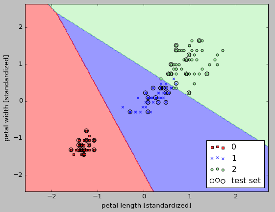
After fitting the model on the training data, we plotted the decision regions, training samples and test samples. Here is the output from the run:
We can predict the class-membership probability of the samples via the predict_proba method.
For example, we can predict the probabilities of the first Iris sample like this:
>>> lr.predict_proba(X_test_std[0,:])This returns the following array:
array([[ 2.05743774e-11, 6.31620264e-02, 9.36837974e-01]])
The array tells us that the model predicts a chance of 93.7 percent that the sample belongs to the Iris-Virginica class, and a 6.3 percent chance that the sample is a Iris-Versicolor flower. We can check the first one is Iris-Virginica class:
>>> y_test
array([2, 1, 0, 2, 0, 2, 0, 1, 1, 1, 2, 1, 1, 1, 1, 0, 1, 1, 0, 0, 2, 1, 0,
       0, 2, 0, 0, 1, 1, 0, 2, 1, 0, 2, 2, 1, 0, 1, 1, 1, 2, 0, 2, 0, 0])
Overfitting is a common problem in machine learning, where a model performs well on training data but does not generalize well to unseen data (test data).
Overfitting occurs when a model is excessively complex, such as having too many parameters relative to the number of observations.
A model that has been overfit has poor predictive performance, as it overreacts to minor fluctuations in the training data.
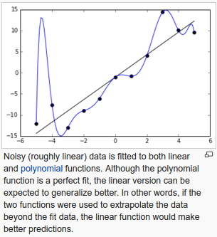
picture from wiki
On the contrary, our model can also suffer from underfitting (high bias), which means that our model is not complex enough to capture the pattern in the training data well and therefore also suffers from low performance on unseen data.
In order to avoid overfitting, it is necessary to use additional techniques (e.g. cross-validation, regularization, early stopping, pruning, or Bayesian priors).
Regularization is a way of finding a good bias-variance tradeoff by tuning the complexity of the model. It is a very useful method to handle collinearity (high correlation among features), filter out noise from data, and eventually prevent overfitting.
The concept behind regularization is to introduce additional information (bias) to penalize extreme parameter weights.
The most common form of regularization is the so-called L2 regularization, which can be written as follows:
$$ \frac {\lambda}{2} {\Vert w \Vert}^2 = \frac {\lambda}{2} \sum_{j=1}^m w_j^2 $$where $\lambda$ is the regularization parameter.
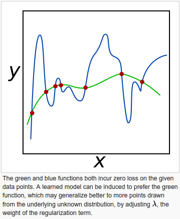
picture from wiki - Regularization
To apply regularization to our logistic regression, we just need to add the regularization term to the cost function to shrink the weights:
$$ J(w) = \left[\sum_i^n -y^{(i)}log(\phi(z^{(i)})-(1-y^{(i)})log(1-\phi(z^{(i)})) \right] + \frac {\lambda}{2} {\Vert w \Vert}^2$$Via the regularization parameter $\lambda$, we can then control how well we fit the training data while keeping the weights small. By increasing the value of $\lambda$ , we increase the regularization strength.
The parameter C that is implemented for the LogisticRegression class in scikit-learn comes from a convention in support vector machines, and C is directly related to the regularization parameter $\lambda$ which is its inverse:
$$ C = \frac {1}{\lambda} $$As we can see in the following plot, the weight coefficients shrink if we decrease the parameter C (increase the regularization strength, $\lambda$):
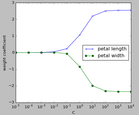
In the picture, we fitted ten logistic regression models with different values for the inverse-regularization parameter C. The code for the plot looks like this:
# scikit-learn logistic regression

from sklearn import datasets
import numpy as np
iris = datasets.load_iris()
X = iris.data[:, [2, 3]]
y = iris.target

from sklearn.model_selection import train_test_split
X_train, X_test, y_train, y_test = train_test_split(X, y, test_size=0.3, random_state=0)

from sklearn.preprocessing import StandardScaler
sc = StandardScaler()
sc.fit(X_train)
X_train_std = sc.transform(X_train)
X_test_std = sc.transform(X_test)

from sklearn.linear_model import LogisticRegression

weights, params = [], []
for c in np.arange(-5, 5):
   lr = LogisticRegression(C=10**c, random_state=0)
   lr.fit(X_train_std, y_train)
   weights.append(lr.coef_[1])
   params.append(10**c)

weights = np.array(weights)

# Decision region drawing
import matplotlib.pyplot as plt

plt.plot(params, weights[:, 0], color='blue', marker='x', label='petal length')
plt.plot(params, weights[:, 1], color='green',  marker='o', label='petal width')
plt.ylabel('weight coefficient')
plt.xlabel('C')
plt.legend(loc='right')
plt.xscale('log')
plt.show()
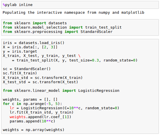
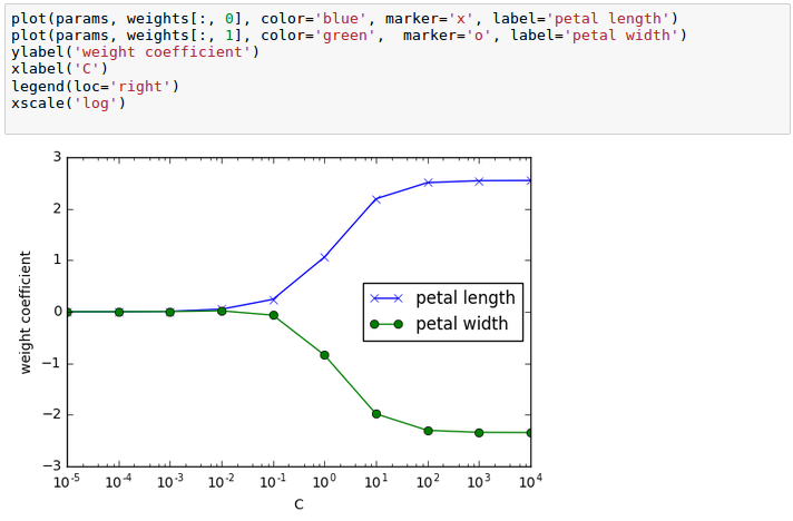
With virtually identical code in Jupyter:
Machine Learning with scikit-learn
scikit-learn installation
scikit-learn : Features and feature extraction - iris dataset
scikit-learn : Machine Learning Quick Preview
scikit-learn : Data Preprocessing I - Missing / Categorical data
scikit-learn : Data Preprocessing II - Partitioning a dataset / Feature scaling / Feature Selection / Regularization
scikit-learn : Data Preprocessing III - Dimensionality reduction vis Sequential feature selection / Assessing feature importance via random forests
Data Compression via Dimensionality Reduction I - Principal component analysis (PCA)
scikit-learn : Data Compression via Dimensionality Reduction II - Linear Discriminant Analysis (LDA)
scikit-learn : Data Compression via Dimensionality Reduction III - Nonlinear mappings via kernel principal component (KPCA) analysis
scikit-learn : Logistic Regression, Overfitting & regularization
scikit-learn : Supervised Learning & Unsupervised Learning - e.g. Unsupervised PCA dimensionality reduction with iris dataset
scikit-learn : Unsupervised_Learning - KMeans clustering with iris dataset
scikit-learn : Linearly Separable Data - Linear Model & (Gaussian) radial basis function kernel (RBF kernel)
scikit-learn : Decision Tree Learning I - Entropy, Gini, and Information Gain
scikit-learn : Decision Tree Learning II - Constructing the Decision Tree
scikit-learn : Random Decision Forests Classification
scikit-learn : Support Vector Machines (SVM)
scikit-learn : Support Vector Machines (SVM) II
Flask with Embedded Machine Learning I : Serializing with pickle and DB setup
Flask with Embedded Machine Learning II : Basic Flask App
Flask with Embedded Machine Learning III : Embedding Classifier
Flask with Embedded Machine Learning IV : Deploy
Flask with Embedded Machine Learning V : Updating the classifier
scikit-learn : Sample of a spam comment filter using SVM - classifying a good one or a bad one
Machine learning algorithms and concepts
Batch gradient descent algorithmSingle Layer Neural Network - Perceptron model on the Iris dataset using Heaviside step activation function
Batch gradient descent versus stochastic gradient descent
Single Layer Neural Network - Adaptive Linear Neuron using linear (identity) activation function with batch gradient descent method
Single Layer Neural Network : Adaptive Linear Neuron using linear (identity) activation function with stochastic gradient descent (SGD)
Logistic Regression
VC (Vapnik-Chervonenkis) Dimension and Shatter
Bias-variance tradeoff
Maximum Likelihood Estimation (MLE)
Neural Networks with backpropagation for XOR using one hidden layer
minHash
tf-idf weight
Natural Language Processing (NLP): Sentiment Analysis I (IMDb & bag-of-words)
Natural Language Processing (NLP): Sentiment Analysis II (tokenization, stemming, and stop words)
Natural Language Processing (NLP): Sentiment Analysis III (training & cross validation)
Natural Language Processing (NLP): Sentiment Analysis IV (out-of-core)
Locality-Sensitive Hashing (LSH) using Cosine Distance (Cosine Similarity)
Artificial Neural Networks (ANN)
[Note] Sources are available at Github - Jupyter notebook files1. Introduction
2. Forward Propagation
3. Gradient Descent
4. Backpropagation of Errors
5. Checking gradient
6. Training via BFGS
7. Overfitting & Regularization
8. Deep Learning I : Image Recognition (Image uploading)
9. Deep Learning II : Image Recognition (Image classification)
10 - Deep Learning III : Deep Learning III : Theano, TensorFlow, and Keras
Python tutorial
Python Home
Introduction
Running Python Programs (os, sys, import)
Modules and IDLE (Import, Reload, exec)
Object Types - Numbers, Strings, and None
Strings - Escape Sequence, Raw String, and Slicing
Strings - Methods
Formatting Strings - expressions and method calls
Files and os.path
Traversing directories recursively
Subprocess Module
Regular Expressions with Python
Regular Expressions Cheat Sheet
Object Types - Lists
Object Types - Dictionaries and Tuples
Functions def, *args, **kargs
Functions lambda
Built-in Functions
map, filter, and reduce
Decorators
List Comprehension
Sets (union/intersection) and itertools - Jaccard coefficient and shingling to check plagiarism
Hashing (Hash tables and hashlib)
Dictionary Comprehension with zip
The yield keyword
Generator Functions and Expressions
generator.send() method
Iterators
Classes and Instances (__init__, __call__, etc.)
if__name__ == '__main__'
argparse
Exceptions
@static method vs class method
Private attributes and private methods
bits, bytes, bitstring, and constBitStream
json.dump(s) and json.load(s)
Python Object Serialization - pickle and json
Python Object Serialization - yaml and json
Priority queue and heap queue data structure
Graph data structure
Dijkstra's shortest path algorithm
Prim's spanning tree algorithm
Closure
Functional programming in Python
Remote running a local file using ssh
SQLite 3 - A. Connecting to DB, create/drop table, and insert data into a table
SQLite 3 - B. Selecting, updating and deleting data
MongoDB with PyMongo I - Installing MongoDB ...
Python HTTP Web Services - urllib, httplib2
Web scraping with Selenium for checking domain availability
REST API : Http Requests for Humans with Flask
Blog app with Tornado
Multithreading ...
Python Network Programming I - Basic Server / Client : A Basics
Python Network Programming I - Basic Server / Client : B File Transfer
Python Network Programming II - Chat Server / Client
Python Network Programming III - Echo Server using socketserver network framework
Python Network Programming IV - Asynchronous Request Handling : ThreadingMixIn and ForkingMixIn
Python Coding Questions I
Python Coding Questions II
Python Coding Questions III
Python Coding Questions IV
Python Coding Questions V
Python Coding Questions VI
Python Coding Questions VII
Python Coding Questions VIII
Python Coding Questions IX
Python Coding Questions X
Image processing with Python image library Pillow
Python and C++ with SIP
PyDev with Eclipse
Matplotlib
Redis with Python
NumPy array basics A
NumPy Matrix and Linear Algebra
Pandas with NumPy and Matplotlib
Celluar Automata
Batch gradient descent algorithm
Longest Common Substring Algorithm
Python Unit Test - TDD using unittest.TestCase class
Simple tool - Google page ranking by keywords
Google App Hello World
Google App webapp2 and WSGI
Uploading Google App Hello World
Python 2 vs Python 3
virtualenv and virtualenvwrapper
Uploading a big file to AWS S3 using boto module
Scheduled stopping and starting an AWS instance
Cloudera CDH5 - Scheduled stopping and starting services
Removing Cloud Files - Rackspace API with curl and subprocess
Checking if a process is running/hanging and stop/run a scheduled task on Windows
Apache Spark 1.3 with PySpark (Spark Python API) Shell
Apache Spark 1.2 Streaming
bottle 0.12.7 - Fast and simple WSGI-micro framework for small web-applications ...
Flask app with Apache WSGI on Ubuntu14/CentOS7 ...
Fabric - streamlining the use of SSH for application deployment
Ansible Quick Preview - Setting up web servers with Nginx, configure enviroments, and deploy an App
Neural Networks with backpropagation for XOR using one hidden layer
NLP - NLTK (Natural Language Toolkit) ...
RabbitMQ(Message broker server) and Celery(Task queue) ...
OpenCV3 and Matplotlib ...
Simple tool - Concatenating slides using FFmpeg ...
iPython - Signal Processing with NumPy
iPython and Jupyter - Install Jupyter, iPython Notebook, drawing with Matplotlib, and publishing it to Github
iPython and Jupyter Notebook with Embedded D3.js
Downloading YouTube videos using youtube-dl embedded with Python
Machine Learning : scikit-learn ...
Django 1.6/1.8 Web Framework ...
Ph.D. / Golden Gate Ave, San Francisco / Seoul National Univ / Carnegie Mellon / UC Berkeley / DevOps / Deep Learning / Visualization