scikit-learn : Data Compression via Dimensionality Reduction II - Linear Discriminant Analysis (LDA)

Linear Discriminant Analysis (LDA) method used to find a linear combination of features that characterizes or separates classes. The resulting combination is used for dimensionality reduction before classification.
Though PCA (unsupervised) attempts to find the orthogonal component axes of maximum variance in a dataset, however, the goal of LDA (supervised) is to find the feature subspace that optimizes class separability.
PCA reduces dimensions by focusing on the data with the most variations. This is useful for the high dimensional data because PCA helps us to draw a simple XY plot.
But we'll use LDA when we're interested maximizing the separability of the data so that we can make the best decisions. In other words, though LDA (supervised) is similar to PCA (unsupervised), but LDA focuses on maximizing the separability among known categories.
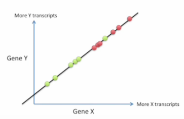
We can tell the difference by the following pictures from Linear Discriminant Analysis (LDA) clearly explained. :
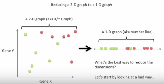
Bad choice first:
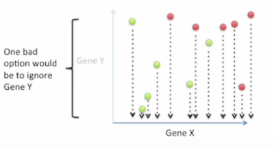
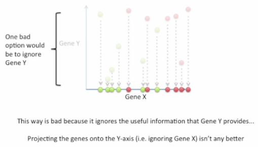
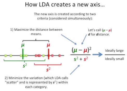
Good choice:
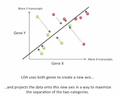
Here is a screen shot how it's done:
The followings are other resources on "PCA" vs "LDA".
The general LDA approach is very similar to a Principal Component Analysis, but in addition to finding the component axes that maximize the variance of our data (PCA), we are additionally interested in the axes that maximize the separation between multiple classes (LDA) - from Linear Discriminant Analysis
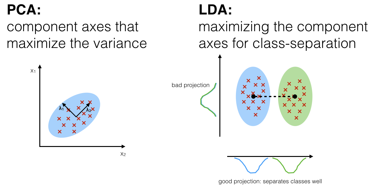
PCA is used as a technique for finding the directions of maximal variance while LDA used as a technique that also cares about class separability (note that, as we can see from the picture, LD2 (y-axis, bad projection) would be a very bad linear discriminant) - What is the difference between LDA and PCA for dimension reduction?
As shown on the x-axis (LD 1), LDA would separate the two normally distributed classes well. Although the y-axis (LD 2) captures a lot of the variance in the dataset, it fails as a good linear discriminant since it does not capture any of the class-discriminatory information.
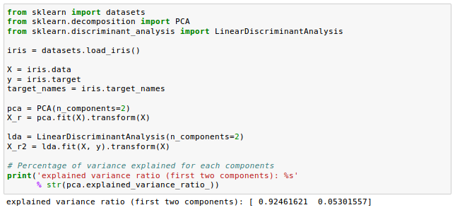
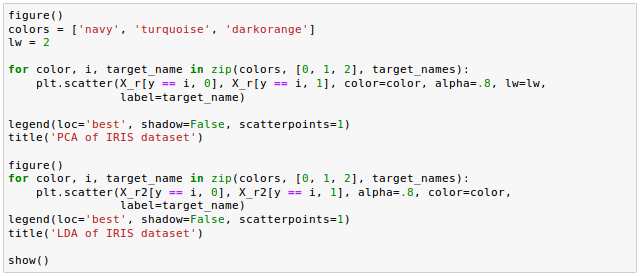
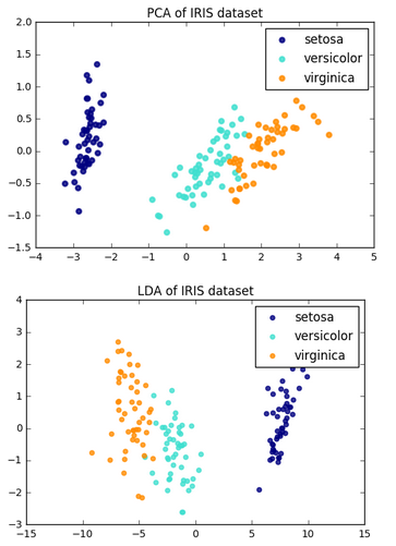
Another comparison from Comparison of LDA and PCA 2D projection of Iris dataset
Let's construct the within-class scatter matrix and between-class scatter matrix.
Each mean vector $m_i$ stores the mean feature value $\mu_m$ with respect to the samples of class $i$: $$ \mathbf m_i = \begin{bmatrix} \mu_{i,alcohol} \\ \mu_{malic acid}\\ \vdots \\ \mu_{proline} \end{bmatrix} \qquad i \in {1,2,3} $$
Here are the key steps of the LDA:
- Standardize the d -dimensional dataset ($d$ is the number of features).
- For each class, compute the $d$-dimensional mean vector.
- Construct the between-class scatter matrix $S_B$ and the within-class scatter
matrix $S_w$.
Using the mean vectors, we can now compute the within-class scatter matrix, $S_w$:
$$ \mathbf S_w = \sum_{i=1}^c \mathbf S_i $$
where the individual scatter matrices individual class $i$ can be given as the following:
$$ \mathbf S_i = \sum_{x \in D_i}^c (\mathbf x-\mathbf m_i)(\mathbf x-\mathbf m_i)^T $$

When we are computing the scatter matrices, we are making an assumption that the class labels in the training set are uniformly distributed. If we print the number of class labels, however, we can see that this assumption is violated:
So, we want to scale the individual scatter matrices $S_i$ before we sum them up as scatter matrix $S_w$. When we divide the scatter matrices by the number of class samples $N_i$, we can see that computing the scatter matrix is in fact the same as computing the covariance matrix $A_i$. The covariance matrix is a normalized version of the scatter matrix: $$ A_i = \frac{1}{N_i}S_W = \frac{1}{N_i} \sum_{x \in D_i}^c (\mathbf x-\mathbf m_i)(\mathbf x-\mathbf m_i)^T $$
After we have computed the scaled within-class scatter matrix (covariance matrix), we can move on to the next step and compute the between-class scatter matrix $S_B$: $$ \mathbf S_B = \sum_{i=1}^c N_i (\mathbf m_i - \mathbf m)(\mathbf m_i - \mathbf m)^T $$ where $m$ is the overall mean that is computed, including samples from all classes.
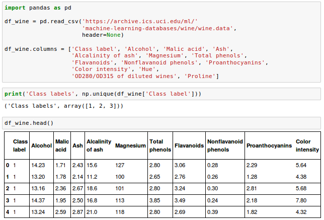

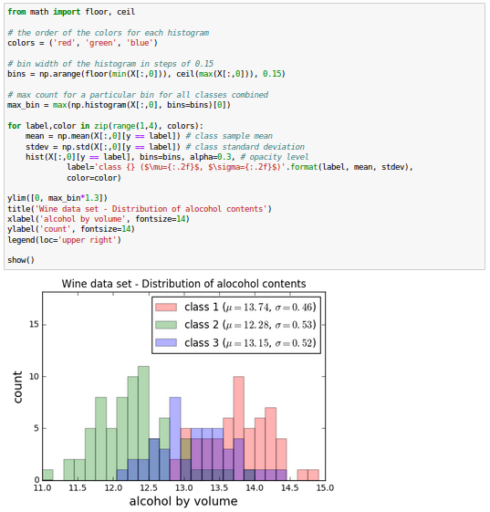
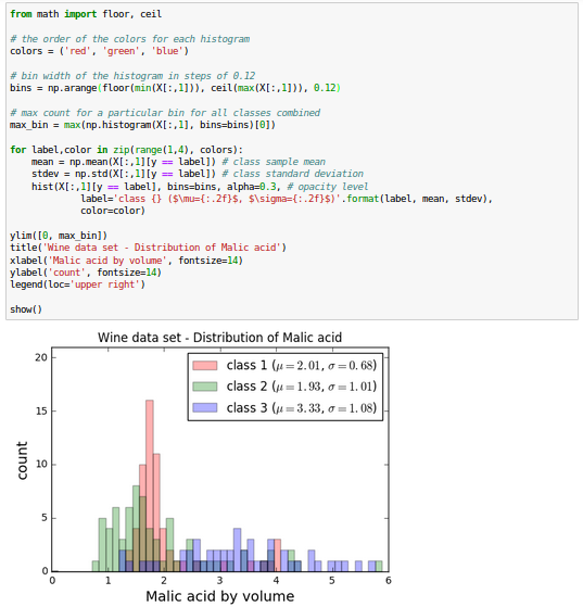
The Wine data looks like this in histogram plots:
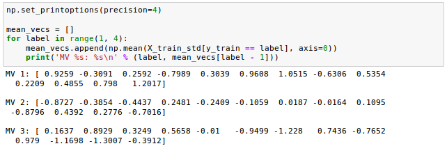
The remaining steps of the LDA are similar to the steps of the PCA. However, instead of performing the eigendecomposition on the covariance matrix, we solve the generalized eigenvalue problem of the matrix $S_w^{-1} S_B$:

Now that we computed the eigen-pairs, we can now sort the eigenvalues in descending order:
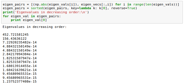
Let's plot the linear discriminants by decreasing eigenvalues similar to the explained variance plot that we created in the PCA section.
From the picture below how much of the class-discriminatory information is captured by the linear discriminants (eigenvectors).
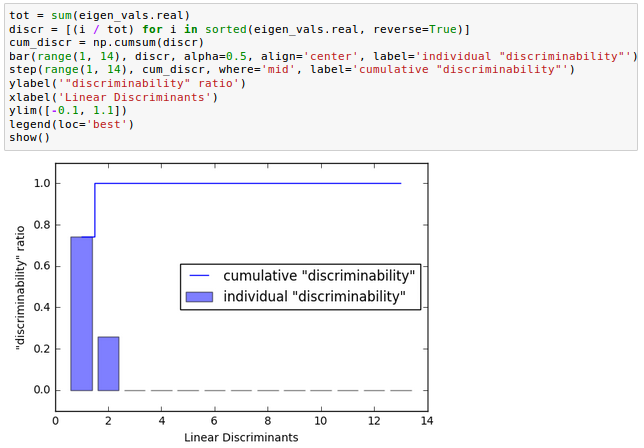
In the picture, we use the content of the class-discriminatory information discriminability, and we can see the first two linear discriminants capture about 100 percent of the useful information in the Wine training dataset:
If we stack the two most discriminative eigenvector columns to create the transformation matrix W, it looks like this:
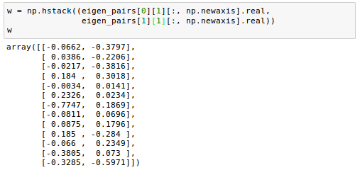
Now we can use the transformation matrix $W$ to transform the training data set by multiplying the matrices:
$$ \mathbf X^\prime = \mathbf X \mathbf W $$
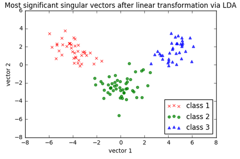
As we can see in the following picture, the three wine classes are now linearly separable in the new feature subspace:
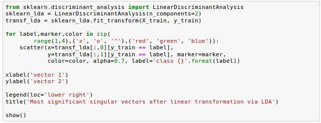
Let's take a look at how LDA class is implemented in scikit-learn.
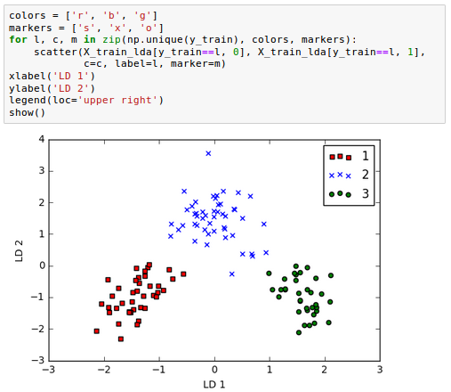
As we can see in the picture below, the logistic regression classifier is able to get a perfect accuracy score for classifying the samples in the test dataset by only using a two-dimensional feature subspace instead of the original 13 Wine features:
Source is available from bogotobogo-Machine-Learning .
Note: This article is mostly based on "Python Machine Learning" by Sebastian Raschka.
Machine Learning with scikit-learn
scikit-learn installation
scikit-learn : Features and feature extraction - iris dataset
scikit-learn : Machine Learning Quick Preview
scikit-learn : Data Preprocessing I - Missing / Categorical data
scikit-learn : Data Preprocessing II - Partitioning a dataset / Feature scaling / Feature Selection / Regularization
scikit-learn : Data Preprocessing III - Dimensionality reduction vis Sequential feature selection / Assessing feature importance via random forests
Data Compression via Dimensionality Reduction I - Principal component analysis (PCA)
scikit-learn : Data Compression via Dimensionality Reduction II - Linear Discriminant Analysis (LDA)
scikit-learn : Data Compression via Dimensionality Reduction III - Nonlinear mappings via kernel principal component (KPCA) analysis
scikit-learn : Logistic Regression, Overfitting & regularization
scikit-learn : Supervised Learning & Unsupervised Learning - e.g. Unsupervised PCA dimensionality reduction with iris dataset
scikit-learn : Unsupervised_Learning - KMeans clustering with iris dataset
scikit-learn : Linearly Separable Data - Linear Model & (Gaussian) radial basis function kernel (RBF kernel)
scikit-learn : Decision Tree Learning I - Entropy, Gini, and Information Gain
scikit-learn : Decision Tree Learning II - Constructing the Decision Tree
scikit-learn : Random Decision Forests Classification
scikit-learn : Support Vector Machines (SVM)
scikit-learn : Support Vector Machines (SVM) II
Flask with Embedded Machine Learning I : Serializing with pickle and DB setup
Flask with Embedded Machine Learning II : Basic Flask App
Flask with Embedded Machine Learning III : Embedding Classifier
Flask with Embedded Machine Learning IV : Deploy
Flask with Embedded Machine Learning V : Updating the classifier
scikit-learn : Sample of a spam comment filter using SVM - classifying a good one or a bad one
Machine learning algorithms and concepts
Batch gradient descent algorithmSingle Layer Neural Network - Perceptron model on the Iris dataset using Heaviside step activation function
Batch gradient descent versus stochastic gradient descent
Single Layer Neural Network - Adaptive Linear Neuron using linear (identity) activation function with batch gradient descent method
Single Layer Neural Network : Adaptive Linear Neuron using linear (identity) activation function with stochastic gradient descent (SGD)
Logistic Regression
VC (Vapnik-Chervonenkis) Dimension and Shatter
Bias-variance tradeoff
Maximum Likelihood Estimation (MLE)
Neural Networks with backpropagation for XOR using one hidden layer
minHash
tf-idf weight
Natural Language Processing (NLP): Sentiment Analysis I (IMDb & bag-of-words)
Natural Language Processing (NLP): Sentiment Analysis II (tokenization, stemming, and stop words)
Natural Language Processing (NLP): Sentiment Analysis III (training & cross validation)
Natural Language Processing (NLP): Sentiment Analysis IV (out-of-core)
Locality-Sensitive Hashing (LSH) using Cosine Distance (Cosine Similarity)
Artificial Neural Networks (ANN)
[Note] Sources are available at Github - Jupyter notebook files1. Introduction
2. Forward Propagation
3. Gradient Descent
4. Backpropagation of Errors
5. Checking gradient
6. Training via BFGS
7. Overfitting & Regularization
8. Deep Learning I : Image Recognition (Image uploading)
9. Deep Learning II : Image Recognition (Image classification)
10 - Deep Learning III : Deep Learning III : Theano, TensorFlow, and Keras
Ph.D. / Golden Gate Ave, San Francisco / Seoul National Univ / Carnegie Mellon / UC Berkeley / DevOps / Deep Learning / Visualization