scikit-learn : Data Preprocessing I - Missing / categorical data

In real-world samples, it is not uncommon that there are missing one or more values such as the blank spaces in our data table.
Quite a few computational tools, however, are unable to handle such missing values and might produce unpredictable results. So, before we proceed with further analyses, it is critical that we take care of those missing values.
To get a better feel for the problem, let's create a simple example using CSV file:
to get a better grasp of the problem: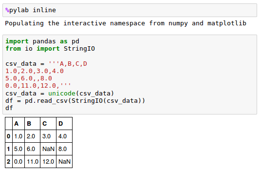
The StringIO() function allows us to read the string assigned to csv_data into a pandas DataFrame via the read_csv() function as if it was a regular CSV file on our hard drive.
Note that the two missing cells were replaced by NaN.
We can use isnull() method to check whether a cell contains a numeric value ( False ) or if data is missing ( True ):
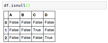
For a larger DataFrame, we may want to use the sum() method which returns the number of missing values per column:

Note that we can always access the underlying NumPy array of the DataFrame via the values attribute before we feed it into a scikit-learn estimator:

So, while scikit-learn was developed for working with NumPy arrays, it can sometimes be more convenient to preprocess data using pandas' DataFrame.
We can remove the corresponding features (columns) or samples (rows) from the dataset.
The rows with missing values can be dropped via the pandas.DataFrame.dropna() method:
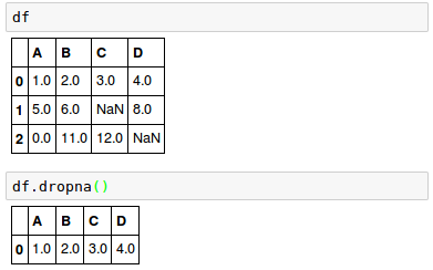
We can drop columns that have at least one NaN in any row by setting the axis argument to 1:
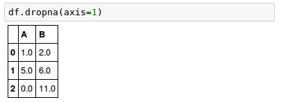
where axis : {0 or 'index', 1 or 'columns'}.
The dropna() method has several additional parameters:
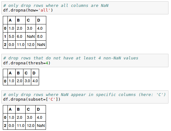
The removal of missing data appears to be a convenient approach, however, it also comes with certain disadvantages:
- There are chances that we may end up removing too many, which will make our analysis not reliable.
- By eliminating too many feature columns, we may run the risk of losing valuable information for our classifier.
In the next section, we will look into interpolation techniques which one of the most commonly used alternatives for dealing with missing data.
Mean imputation is a method replacing the missing values with the mean value of the entire feature column. While this method maintains the sample size and is easy to use, the variability in the data is reduced, so the standard deviations and the variance estimates tend to be underestimated.
We'll use the sklearn.preprocessing.Imputer class:
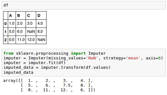
Here, we replaced each NaN value by the corresponding mean from each feature column.
We can use the row means if we change the setting axis=0 to axis=1:

As for the strategy parameter, there are other options such as median or most_frequent.
The Imputer class we used in the previous section belongs to the so-called transformer classes in scikit-learn that are used for data transformation.
There are two methods of estimators:
- fit:
This method is used to learn the parameters from the training data. - transform:
transform() method uses those parameters to transform the data.
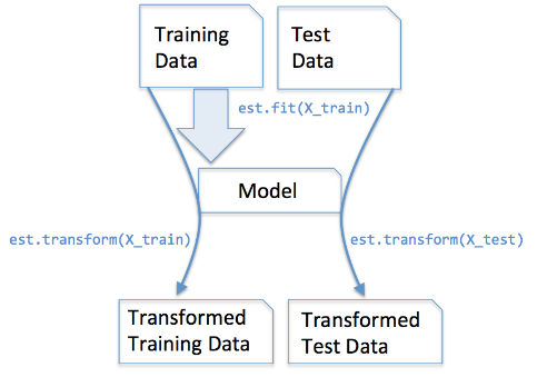
The diagram below shows how a transformer fitted on the training data is used to transform a training dataset as well as a new test dataset:
In supervised learning tasks, we additionally provide the class labels for fitting the model, which can then be used to make predictions about new data samples via the predict() method:
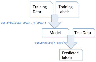
picture source : Python machine learning by Sebastian Raschka
Not all data has numerical values. Here are examples of categorical data:
- The blood type of a person: A, B, AB or O.
- The state that a resident of the United States lives in.
- T-shirt size. XL > L > M
- T-shirt color.
Even among categorical data, we may want to distinguish further between nominal and ordinal which can be sorted or ordered features. So, T-shirt size can be an ordinal feature, because we can define an order XL > L > M.
Let's create a new categorical data frame:
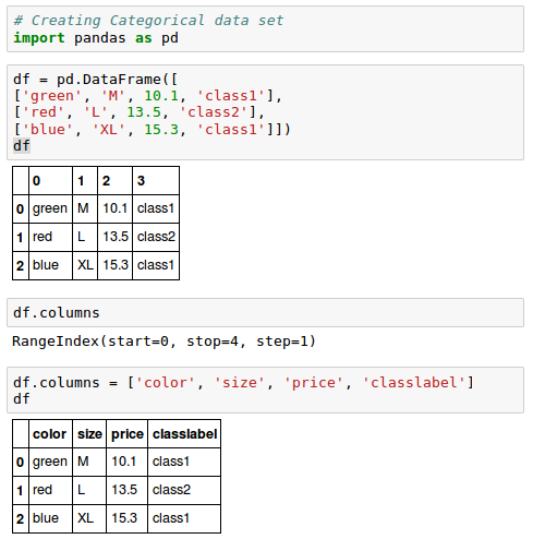
As we can see from the output, the DataFrame contains a nominal feature (color), an ordinal feature (size) as well as a numerical feature (price) column. In the last column, the class labels are created.
In order for out learning algorithm to interpret the ordinal features correctly, we should convert the categorical string values into integers.
However, since there is no convenient function that can automatically derive the correct order of the labels of our size feature, we have to define the mapping manually.
Let's assume that we know the difference between features such as XL = L + 1 = M + 2.
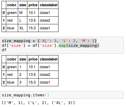
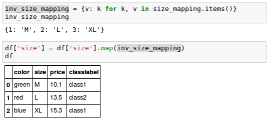
If we want to transform the integer values back to the original string representation, we can simply define a reverse-mapping dictionary "inv_size_mapping" that can then be used via the pandas' map method on the transformed feature column similar to the "size_mapping" dictionary that we used previously:
Usually, class labels are required to be encoded as integer values.
While most estimators for classification in scikit-learn convert class labels to integers internally, as a good practice, we may want to provide class labels as integer arrays to avoid any issues.
To encode the class labels, we can use an approach similar to the mapping of ordinal features discussed in the previous section.
Since class labels are not ordinal, it doesn't matter which integer number we assign to a particular string-label.
So, we can simply enumerate the class labels starting at 0:

Now we want mapping dictionary to transform the class labels into integers:
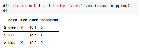
As we did for "size" in the previous section, we can reverse the key-value pairs in the mapping dictionary as follows to map the converted class labels back to the original string representation:
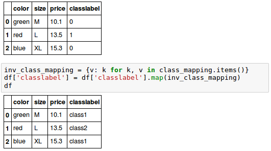
Though we encoded the class labels manually, luckily, there is a convenient LabelEncoder class directly implemented in scikit-learn to achieve the same:

Note that the fit_transform() method is just a shortcut for calling fit and transform separately, and we can use the inverse_transform() method to transform the integer class labels back into their original string representation:

So far, we used a simple dictionary-mapping approach to convert the ordinal size feature into integers.
Because scikit-learn's estimators treat class labels without any order, we used the convenient LabelEncoder class to encode the string labels into integers.
We can use a similar approach to transform the nominal color column of our dataset as well:
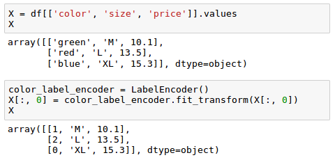
We may want to create a new dummy feature for each unique value in the nominal feature column. In other words, we would convert the color feature into three new features: blue, green, and red. Binary values can then be used to indicate the particular color of a sample; for example, a blue sample can be encoded as blue=1, green=0, red=0. This technique is called one-hot encoding.
In order to perform this transformation, we can use the scikit-learn.preprocessingOneHotEncoder:
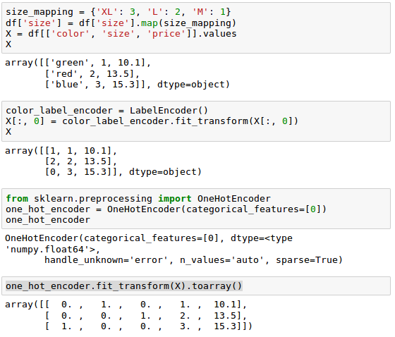
Note that when we initialized the OneHotEncoder, we defined the column position of the variable that we want to transform via the categorical_features parameter which is the first column in the feature matrix X.
The OneHotEncoder, by default, returns a sparse matrix when we use the transform() method, and we converted the sparse matrix representation into a regular (dense) NumPy array for the purposes of visualization via the toarray() method. Sparse matrices are simply a more efficient way of storing large datasets, and one that is supported by many scikit-learn functions. It is especially useful if it contains a lot of zeros.
If we want to omit the toarray() step, we may initialize the encoder as OneHotEncoder(...,sparse=False) to return a regular NumPy array:

Another way which is more convenient is to create those dummy features via one-hot encoding is to use the pandas.get_dummies() method. Applied on a DataFrame, the get_dummies() method will only convert string columns and leave all other columns unchanged:

Source is available from bogotobogo-Machine-Learning .
Next:
Data Preprocessing II - Partitioning a dataset / Feature scaling / Feature Selection / RegularizationMachine Learning with scikit-learn
scikit-learn installation
scikit-learn : Features and feature extraction - iris dataset
scikit-learn : Machine Learning Quick Preview
scikit-learn : Data Preprocessing I - Missing / Categorical data
scikit-learn : Data Preprocessing II - Partitioning a dataset / Feature scaling / Feature Selection / Regularization
scikit-learn : Data Preprocessing III - Dimensionality reduction vis Sequential feature selection / Assessing feature importance via random forests
Data Compression via Dimensionality Reduction I - Principal component analysis (PCA)
scikit-learn : Data Compression via Dimensionality Reduction II - Linear Discriminant Analysis (LDA)
scikit-learn : Data Compression via Dimensionality Reduction III - Nonlinear mappings via kernel principal component (KPCA) analysis
scikit-learn : Logistic Regression, Overfitting & regularization
scikit-learn : Supervised Learning & Unsupervised Learning - e.g. Unsupervised PCA dimensionality reduction with iris dataset
scikit-learn : Unsupervised_Learning - KMeans clustering with iris dataset
scikit-learn : Linearly Separable Data - Linear Model & (Gaussian) radial basis function kernel (RBF kernel)
scikit-learn : Decision Tree Learning I - Entropy, Gini, and Information Gain
scikit-learn : Decision Tree Learning II - Constructing the Decision Tree
scikit-learn : Random Decision Forests Classification
scikit-learn : Support Vector Machines (SVM)
scikit-learn : Support Vector Machines (SVM) II
Flask with Embedded Machine Learning I : Serializing with pickle and DB setup
Flask with Embedded Machine Learning II : Basic Flask App
Flask with Embedded Machine Learning III : Embedding Classifier
Flask with Embedded Machine Learning IV : Deploy
Flask with Embedded Machine Learning V : Updating the classifier
scikit-learn : Sample of a spam comment filter using SVM - classifying a good one or a bad one
Machine learning algorithms and concepts
Batch gradient descent algorithmSingle Layer Neural Network - Perceptron model on the Iris dataset using Heaviside step activation function
Batch gradient descent versus stochastic gradient descent
Single Layer Neural Network - Adaptive Linear Neuron using linear (identity) activation function with batch gradient descent method
Single Layer Neural Network : Adaptive Linear Neuron using linear (identity) activation function with stochastic gradient descent (SGD)
Logistic Regression
VC (Vapnik-Chervonenkis) Dimension and Shatter
Bias-variance tradeoff
Maximum Likelihood Estimation (MLE)
Neural Networks with backpropagation for XOR using one hidden layer
minHash
tf-idf weight
Natural Language Processing (NLP): Sentiment Analysis I (IMDb & bag-of-words)
Natural Language Processing (NLP): Sentiment Analysis II (tokenization, stemming, and stop words)
Natural Language Processing (NLP): Sentiment Analysis III (training & cross validation)
Natural Language Processing (NLP): Sentiment Analysis IV (out-of-core)
Locality-Sensitive Hashing (LSH) using Cosine Distance (Cosine Similarity)
Artificial Neural Networks (ANN)
[Note] Sources are available at Github - Jupyter notebook files1. Introduction
2. Forward Propagation
3. Gradient Descent
4. Backpropagation of Errors
5. Checking gradient
6. Training via BFGS
7. Overfitting & Regularization
8. Deep Learning I : Image Recognition (Image uploading)
9. Deep Learning II : Image Recognition (Image classification)
10 - Deep Learning III : Deep Learning III : Theano, TensorFlow, and Keras
Ph.D. / Golden Gate Ave, San Francisco / Seoul National Univ / Carnegie Mellon / UC Berkeley / DevOps / Deep Learning / Visualization