Single Layer Neural Network : Adaptive Linear Neuron using linear (identity) activation function with stochastic gradient descent (SGD)
In Single Layer Neural Network - Adaptive Linear Neuron using linear (identity) activation function with batch gradient descent method, we minimized a cost function (objective function) by taking a step into the opposite direction of a gradient that is calculated from the whole training set with batch gradient descent.
Running batch gradient descent with a huge data set can be very costly because we need to reevaluate the whole training dataset each time step.
One of the popular alternative to the batch gradient descent algorithm is stochastic gradient descent (SGD), also known as incremental gradient descent.
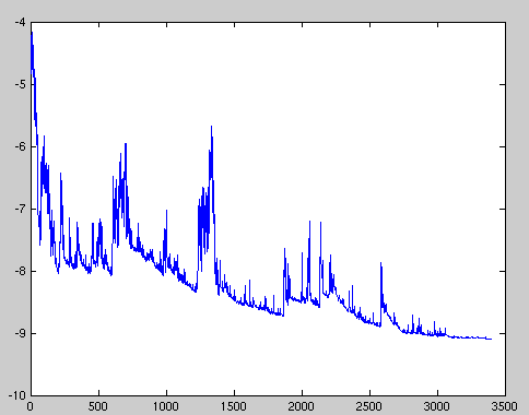
The picture below (Stochastic gradient descent -wiki) is the typical result from SGD:

Fluctuations in the total objective function as gradient steps with respect to mini-batches are taken.
In our previous tutorial (Single Layer Neural Network - Adaptive Linear Neuron using linear (identity) activation function with batch gradient descent method), we calculated the weights based on the sum of the accumulated errors over all samples $x^{(i)}$ like this:
$$ \Delta w = \eta \sum_i (y^{(i)}-\phi(z^{(i)}))x^{(i)}$$With SGD, we update the weights incrementally for each training sample:
$$ \eta (y^{(i)}-\phi(z^{(i)}))x^{(i)}$$Stochastic gradient descent (SGD) is an approximation of gradient descent, however, it usualy reaches convergence much faster because of the more frequent weight updates.
Since each gradient is calculated based on a single training example, as shown in the sample of the previous section, the error is noisier than in gradient descent, which can also have the advantage that stochastic gradient descent can escape shallow local minima more readily.
To obtain accurate results via stochastic gradient descent, it is important to present it with data in a random order, which is why we want to shuffle the training set for every epoch to prevent cycles.
Here are the steps of SGD in pseudo code:
- Choose an initial vector of parameters $w$ and learning rate $\eta$.
- Repeat until an approximate minimum is obtained:
- Randomly shuffle examples in the training set.
- For $i=1,2,...,n$ do: $$w:=w-\eta \nabla J_i(w)$$ where $J$ is a cost function
Since we've already implemented using gradient descent (Single Layer Neural Network - Adaptive Linear Neuron using linear (identity) activation function with batch gradient descent method), we only need to make a few adjustments to the existing learning algorithm to update the weights via stochastic gradient descent.
Inside the fit method, we will now update the weights after each training sample.
Furthermore, we will implement an additional partial_fit method, which does not reinitialize the weights, for on-line learning.
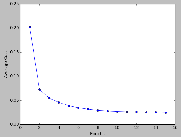
In order to check if our algorithm converged after training, we will calculate the cost as the average cost of the training samples in each iteration.
Also, we will shuffle the training data before each epoch to avoid cycles when we are optimizing the cost function via the random_state parameter.
Here is the source code using SGD:
from matplotlib.colors import ListedColormap
import matplotlib.pyplot as plt
import numpy as np
from numpy.random import seed
import pandas as pd

# Stochastic Gradient Descent
class SGD(object):
   def __init__(self, rate = 0.01, niter = 10,
                shuffle=True, random_state=None):
      self.rate = rate
      self.niter = niter
      self.weight_initialized = False

      # If True, Shuffles training data every epoch
      self.shuffle = shuffle

      # Set random state for shuffling and initializing the weights.
      if random_state:
         seed(random_state)

   def fit(self, X, y):
      """Fit training data
      X : Training vectors, X.shape : [#samples, #features]
      y : Target values, y.shape : [#samples]
      """

      # weights
      self.initialize_weights(X.shape[1])

      # Cost function
      self.cost = []

      for i in range(self.niter):
         if self.shuffle:
            X, y = self.shuffle_set(X, y)
         cost = []
         for xi, target in zip(X, y):
            cost.append(self.update_weights(xi, target))
         avg_cost = sum(cost)/len(y)
         self.cost.append(avg_cost)
      return self

   def partial_fit(self, X, y):
      """Fit training data without reinitializing the weights"""
      if not self.weight_initialized:
         self.initialize_weights(X.shape[1])
      if y.ravel().shape[0] > 1:
         for xi, target in zip(X, y):
            self.update_weights(xi, target)
      else:
         self.up
      return self

   def shuffle_set(self, X, y):
      """Shuffle training data"""
      r = np.random.permutation(len(y))
      return X[r], y[r]

   def initialize_weights(self, m):
      """Initialize weights to zeros"""
      self.weight = np.zeros(1 + m)
      self.weight_initialized = True

   def update_weights(self, xi, target):
      """Apply SGD learning rule to update the weights"""
      output = self.net_input(xi)
      error = (target - output)
      self.weight[1:] += self.rate * xi.dot(error)
      self.weight[0] += self.rate * error
      cost = 0.5 * error**2
      return cost

   def net_input(self, X):
      """Calculate net input"""
      return np.dot(X, self.weight[1:]) + self.weight[0]

   def activation(self, X):
      """Compute linear activation"""
      return self.net_input(X)

   def predict(self, X):
      """Return class label after unit step"""
      return np.where(self.activation(X) >= 0.0, 1, -1)

def plot_decision_regions(X, y, classifier, resolution=0.02):
   # setup marker generator and color map
   markers = ('s', 'x', 'o', '^', 'v')
   colors = ('red', 'blue', 'lightgreen', 'gray', 'cyan')
   cmap = ListedColormap(colors[:len(np.unique(y))])

   # plot the decision surface
   x1_min, x1_max = X[:,  0].min() - 1, X[:, 0].max() + 1
   x2_min, x2_max = X[:, 1].min() - 1, X[:, 1].max() + 1
   xx1, xx2 = np.meshgrid(np.arange(x1_min, x1_max, resolution),
   np.arange(x2_min, x2_max, resolution))
   Z = classifier.predict(np.array([xx1.ravel(), xx2.ravel()]).T)
   Z = Z.reshape(xx1.shape)
   plt.contourf(xx1, xx2, Z, alpha=0.4, cmap=cmap)
   plt.xlim(xx1.min(), xx1.max())
   plt.ylim(xx2.min(), xx2.max())

   # plot class samples
   for idx, cl in enumerate(np.unique(y)):
      plt.scatter(x=X[y == cl, 0], y=X[y == cl, 1],
      alpha=0.8, c=cmap(idx),
      marker=markers[idx], label=cl)

df = pd.read_csv('https://archive.ics.uci.edu/ml/machine-learning-databases/iris/iris.data', header=None)

y = df.iloc[0:100, 4].values
y = np.where(y == 'Iris-setosa', -1, 1)
X = df.iloc[0:100, [0, 2]].values

# standardize
X_std = np.copy(X)
X_std[:,0] = (X[:,0] - X[:,0].mean()) / X[:,0].std()
X_std[:,1] = (X[:,1] - X[:,1].mean()) / X[:,1].std()

sgd = SGD(niter=15, rate=0.01, random_state=1)
sgd.fit(X_std, y)
plot_decision_regions(X_std, y, classifier=sgd)
plt.title('SGD - Stochastic Gradient Descent')
plt.xlabel('sepal length [standardized]')
plt.ylabel('petal length [standardized]')
plt.legend(loc='upper left')
plt.show()
plt.plot(range(1, len(sgd.cost) + 1), sgd.cost, marker='o')
plt.xlabel('Epochs')
plt.ylabel('Average Cost')
plt.show()
The np.random.permutationpermutation function in suffle_set() generates a random sequence of unique numbers in the range 0 to 100.


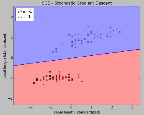
As we can see from the pictures, the average cost goes down pretty quickly, and the final decision boundary after 15 epochs looks similar to the results from batch gradient descent in previous tutorial.
If we want to update our model via on-line learning scenario with streaming data, we can simply call the partial_fit method on individual samples:
sgd.partial_fit(X_std[0, :], y[0])
Machine Learning with scikit-learn
scikit-learn installation
scikit-learn : Features and feature extraction - iris dataset
scikit-learn : Machine Learning Quick Preview
scikit-learn : Data Preprocessing I - Missing / Categorical data
scikit-learn : Data Preprocessing II - Partitioning a dataset / Feature scaling / Feature Selection / Regularization
scikit-learn : Data Preprocessing III - Dimensionality reduction vis Sequential feature selection / Assessing feature importance via random forests
Data Compression via Dimensionality Reduction I - Principal component analysis (PCA)
scikit-learn : Data Compression via Dimensionality Reduction II - Linear Discriminant Analysis (LDA)
scikit-learn : Data Compression via Dimensionality Reduction III - Nonlinear mappings via kernel principal component (KPCA) analysis
scikit-learn : Logistic Regression, Overfitting & regularization
scikit-learn : Supervised Learning & Unsupervised Learning - e.g. Unsupervised PCA dimensionality reduction with iris dataset
scikit-learn : Unsupervised_Learning - KMeans clustering with iris dataset
scikit-learn : Linearly Separable Data - Linear Model & (Gaussian) radial basis function kernel (RBF kernel)
scikit-learn : Decision Tree Learning I - Entropy, Gini, and Information Gain
scikit-learn : Decision Tree Learning II - Constructing the Decision Tree
scikit-learn : Random Decision Forests Classification
scikit-learn : Support Vector Machines (SVM)
scikit-learn : Support Vector Machines (SVM) II
Flask with Embedded Machine Learning I : Serializing with pickle and DB setup
Flask with Embedded Machine Learning II : Basic Flask App
Flask with Embedded Machine Learning III : Embedding Classifier
Flask with Embedded Machine Learning IV : Deploy
Flask with Embedded Machine Learning V : Updating the classifier
scikit-learn : Sample of a spam comment filter using SVM - classifying a good one or a bad one
Machine learning algorithms and concepts
Batch gradient descent algorithmSingle Layer Neural Network - Perceptron model on the Iris dataset using Heaviside step activation function
Batch gradient descent versus stochastic gradient descent
Single Layer Neural Network - Adaptive Linear Neuron using linear (identity) activation function with batch gradient descent method
Single Layer Neural Network : Adaptive Linear Neuron using linear (identity) activation function with stochastic gradient descent (SGD)
Logistic Regression
VC (Vapnik-Chervonenkis) Dimension and Shatter
Bias-variance tradeoff
Maximum Likelihood Estimation (MLE)
Neural Networks with backpropagation for XOR using one hidden layer
minHash
tf-idf weight
Natural Language Processing (NLP): Sentiment Analysis I (IMDb & bag-of-words)
Natural Language Processing (NLP): Sentiment Analysis II (tokenization, stemming, and stop words)
Natural Language Processing (NLP): Sentiment Analysis III (training & cross validation)
Natural Language Processing (NLP): Sentiment Analysis IV (out-of-core)
Locality-Sensitive Hashing (LSH) using Cosine Distance (Cosine Similarity)
Artificial Neural Networks (ANN)
[Note] Sources are available at Github - Jupyter notebook files1. Introduction
2. Forward Propagation
3. Gradient Descent
4. Backpropagation of Errors
5. Checking gradient
6. Training via BFGS
7. Overfitting & Regularization
8. Deep Learning I : Image Recognition (Image uploading)
9. Deep Learning II : Image Recognition (Image classification)
10 - Deep Learning III : Deep Learning III : Theano, TensorFlow, and Keras
Ph.D. / Golden Gate Ave, San Francisco / Seoul National Univ / Carnegie Mellon / UC Berkeley / DevOps / Deep Learning / Visualization