Artificial Neural Network (ANN) 7 - Overfitting & Regularization
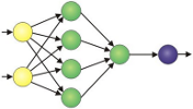
Continued from Artificial Neural Network (ANN) 6 - Training via BFGS where we trained our neural network via BFGS
We saw our neural network gave a pretty good predictions of our test score based on how many hours we slept, and how many hours we studied the night before.
In this article, we want to check how well our model reflects the real world data.
We want our model to fit the signal but not the noise so that we should be able to avoid overfitting.
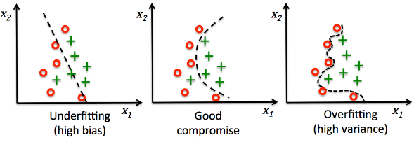
picture source : Python machine learning by Sebastian Raschka
First, we'll work on diagnosing overfitting, and then we'll work on fixing it.
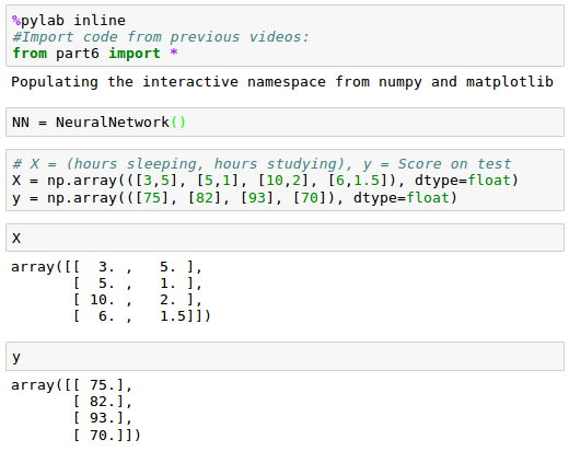
Let's start with an input data for training our neural network:
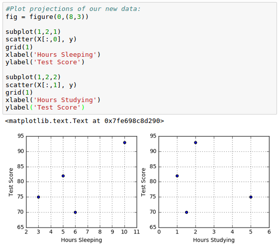
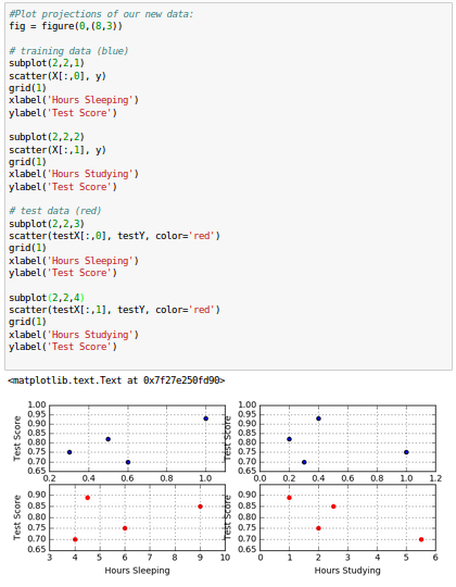
Here is the plot for our input data, scores vs hours of sleep/study:
To train our model, we need to normalize training data:
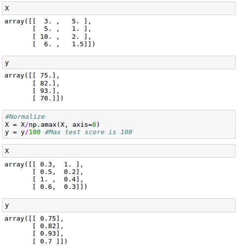
Let's start training our network with the normalized data set:

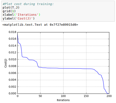
The cost function ($J$) plot vs iterations looks like this:
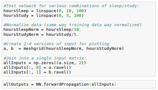
Now we want to generate more data using "numpy.linspace()":
Contour for the newly generated data looks like this:
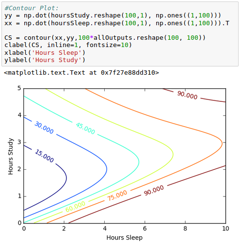
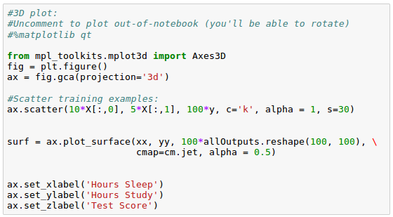
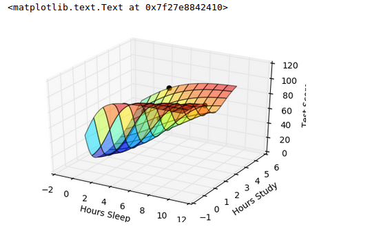
From the picture, we can see our model is overfitting, but how do we know for sure?
In general, we want to split our data into 2 portions: training and testing. We won't touch our testing data while training the model, and only use it to see how we're doing since our testing data is a simulation of the real world.
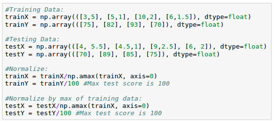
We may want to modify Trainer class a bit to check testing error during training:
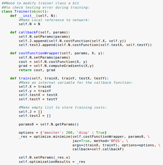
Let's train our model with the new data:
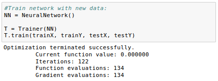
We can plot the error on our training and testing sets as we train our model and identify the exact point at which overfitting begins.
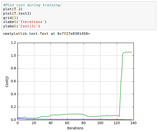
As we can see from the picture above, our cost function ($\color{green}{J}$) with real data(test) soars around it=125 while the $\color{blue}{J}$ with training data continues to become smaller and smaller.
Now we know we have overfitting issue, but how do we fix it?
A simple rule of thumb is that we should have at least 10 times as many examples as the degrees for freedom in our model. For us, since we have 9 weights that can change, we would need 90 observations, which we certainly don't have.
One of th popular and effective ways of mitigating the overfitting issue is to use a technique called regularization.
One way to implement regularization is to add a term to our cost function that penalizes overly complex models.
A simple, but effective way to do this is to add together the square of our weights to our cost function so that models with larger magnitudes of weights, cost more.
We'll need to normalize the other part of our cost function to ensure that our ratio of the two error terms does not change with respect to the number of examples.
We're going to introduce a regularization hyper parameter, $\lambda$, that will allow us to tune the relative cost. So, higher values of lambda will impose bigger penalties for high model complexity.
We need to make changes to costFunction and costFunctionPrime as well as the __init__():
#New complete class, with changes:
class NeuralNetwork(object):
    def __init__(self, Lambda=0):
        #Define Hyperparameters
        self.inputLayerSize = 2
        self.outputLayerSize = 1
        self.hiddenLayerSize = 3

        #Weights (parameters)
        self.W1 = np.random.randn(self.inputLayerSize,self.hiddenLayerSize)
        self.W2 = np.random.randn(self.hiddenLayerSize,self.outputLayerSize)

        #Regularization Parameter:
        self.Lambda = Lambda

    def forwardPropagation(self, X):
        #Propogate inputs though network
        self.z2 = np.dot(X, self.W1)
        self.a2 = self.sigmoid(self.z2)
        self.z3 = np.dot(self.a2, self.W2)
        yHat = self.sigmoid(self.z3)
        return yHat

    def sigmoid(self, z):
        #Apply sigmoid activation function to scalar, vector, or matrix
        return 1/(1+np.exp(-z))

    def sigmoidPrime(self,z):
        #Gradient of sigmoid
        return np.exp(-z)/((1+np.exp(-z))**2)

    def costFunction(self, X, y):
        #Compute cost for given X,y, use weights already stored in class.
        self.yHat = self.forwardPropagation(X)
        J = 0.5*sum((y-self.yHat)**2)/X.shape[0] + (self.Lambda/2)*(np.sum(self.W1**2)+np.sum(self.W2**2))
        return J

    def costFunctionPrime(self, X, y):
        #Compute derivative with respect to W and W2 for a given X and y:
        self.yHat = self.forwardPropagation(X)

        delta3 = np.multiply(-(y-self.yHat), self.sigmoidPrime(self.z3))
        #Add gradient of regularization term:
        dJdW2 = np.dot(self.a2.T, delta3)/X.shape[0] +  self.Lambda*self.W2

        delta2 = np.dot(delta3, self.W2.T)*self.sigmoidPrime(self.z2)
        #Add gradient of regularization term:
        dJdW1 = np.dot(X.T, delta2)/X.shape[0] + self.Lambda*self.W1

        return dJdW1, dJdW2

    #Helper functions for interacting with other methods/classes
    def getParams(self):
        #Get W1 and W2 Rolled into vector:
        params = np.concatenate((self.W1.ravel(), self.W2.ravel()))
        return params

    def setParams(self, params):
        #Set W1 and W2 using single parameter vector:
        W1_start = 0
        W1_end = self.hiddenLayerSize*self.inputLayerSize
        self.W1 = np.reshape(params[W1_start:W1_end], \
                             (self.inputLayerSize, self.hiddenLayerSize))
        W2_end = W1_end + self.hiddenLayerSize*self.outputLayerSize
        self.W2 = np.reshape(params[W1_end:W2_end], \
                             (self.hiddenLayerSize, self.outputLayerSize))

    def computeGradients(self, X, y):
        dJdW1, dJdW2 = self.costFunctionPrime(X, y)
        return np.concatenate((dJdW1.ravel(), dJdW2.ravel()))
Since we made some changes, let's make sure our gradients are correct after making those changes:
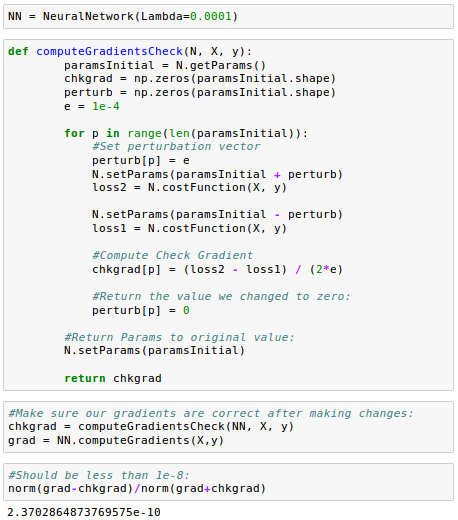
Let's train our model again.
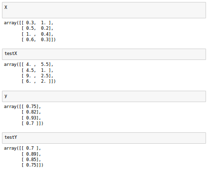
Here is the data set we're going to use:
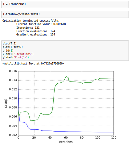
Now our training and testing errors are much closer, which is the indication of the success in reducing the overfit on this dataset.
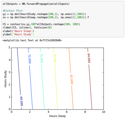
Let's see our contour plot for test scores against sleep/study hours:
3-D plot:
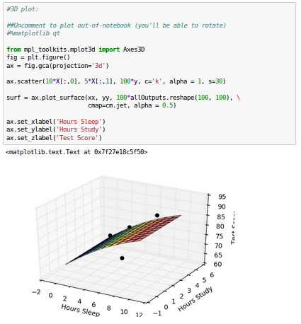
While we see that the fit is still good, but our model is no longer that interested in the fitting accuracy to our data.
To reduce the overfitting further, we may want to increase the regularization parameter, $\lambda$.
Here is the plot of the 6 weights ($W^{(1)}$) for hidden layer and 3 weights ($W^{(2)}$) for output layer of our neural network:
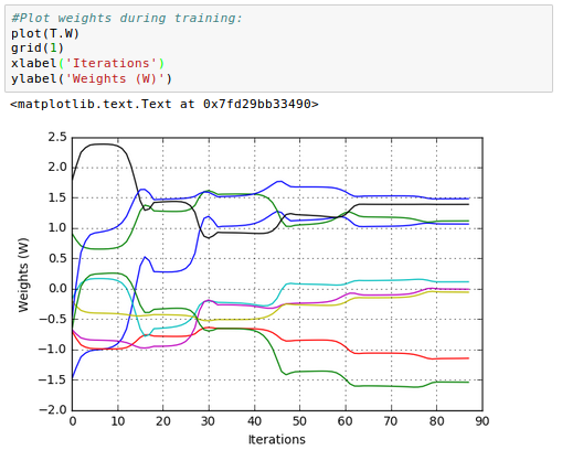
Note: this picture for weights update was plotted later from a separated run. So, it does not reflect the pictures in the previous section though it shows the general trend how the weight are updated during the iterations.
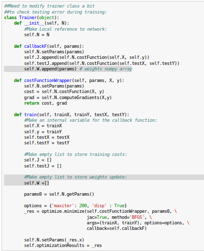
To get the $W$, we need to modify the lines highlighted in our Trainer class as shown below:
Please visit Github Artificial-Neural-Networks-with-Jupyter .
Next:
8. Artificial Neural Network (ANN) 8 - Deep Learning I : Image Recognition (Image uploading)Machine Learning with scikit-learn
scikit-learn installation
scikit-learn : Features and feature extraction - iris dataset
scikit-learn : Machine Learning Quick Preview
scikit-learn : Data Preprocessing I - Missing / Categorical data
scikit-learn : Data Preprocessing II - Partitioning a dataset / Feature scaling / Feature Selection / Regularization
scikit-learn : Data Preprocessing III - Dimensionality reduction vis Sequential feature selection / Assessing feature importance via random forests
Data Compression via Dimensionality Reduction I - Principal component analysis (PCA)
scikit-learn : Data Compression via Dimensionality Reduction II - Linear Discriminant Analysis (LDA)
scikit-learn : Data Compression via Dimensionality Reduction III - Nonlinear mappings via kernel principal component (KPCA) analysis
scikit-learn : Logistic Regression, Overfitting & regularization
scikit-learn : Supervised Learning & Unsupervised Learning - e.g. Unsupervised PCA dimensionality reduction with iris dataset
scikit-learn : Unsupervised_Learning - KMeans clustering with iris dataset
scikit-learn : Linearly Separable Data - Linear Model & (Gaussian) radial basis function kernel (RBF kernel)
scikit-learn : Decision Tree Learning I - Entropy, Gini, and Information Gain
scikit-learn : Decision Tree Learning II - Constructing the Decision Tree
scikit-learn : Random Decision Forests Classification
scikit-learn : Support Vector Machines (SVM)
scikit-learn : Support Vector Machines (SVM) II
Flask with Embedded Machine Learning I : Serializing with pickle and DB setup
Flask with Embedded Machine Learning II : Basic Flask App
Flask with Embedded Machine Learning III : Embedding Classifier
Flask with Embedded Machine Learning IV : Deploy
Flask with Embedded Machine Learning V : Updating the classifier
scikit-learn : Sample of a spam comment filter using SVM - classifying a good one or a bad one
Machine learning algorithms and concepts
Batch gradient descent algorithmSingle Layer Neural Network - Perceptron model on the Iris dataset using Heaviside step activation function
Batch gradient descent versus stochastic gradient descent
Single Layer Neural Network - Adaptive Linear Neuron using linear (identity) activation function with batch gradient descent method
Single Layer Neural Network : Adaptive Linear Neuron using linear (identity) activation function with stochastic gradient descent (SGD)
Logistic Regression
VC (Vapnik-Chervonenkis) Dimension and Shatter
Bias-variance tradeoff
Maximum Likelihood Estimation (MLE)
Neural Networks with backpropagation for XOR using one hidden layer
minHash
tf-idf weight
Natural Language Processing (NLP): Sentiment Analysis I (IMDb & bag-of-words)
Natural Language Processing (NLP): Sentiment Analysis II (tokenization, stemming, and stop words)
Natural Language Processing (NLP): Sentiment Analysis III (training & cross validation)
Natural Language Processing (NLP): Sentiment Analysis IV (out-of-core)
Locality-Sensitive Hashing (LSH) using Cosine Distance (Cosine Similarity)
Artificial Neural Networks (ANN)
[Note] Sources are available at Github - Jupyter notebook files1. Introduction
2. Forward Propagation
3. Gradient Descent
4. Backpropagation of Errors
5. Checking gradient
6. Training via BFGS
7. Overfitting & Regularization
8. Deep Learning I : Image Recognition (Image uploading)
9. Deep Learning II : Image Recognition (Image classification)
10 - Deep Learning III : Deep Learning III : Theano, TensorFlow, and Keras
Ph.D. / Golden Gate Ave, San Francisco / Seoul National Univ / Carnegie Mellon / UC Berkeley / DevOps / Deep Learning / Visualization