scikit-learn : Data Preprocessing III - Dimensionality reduction via Sequential feature selection / Assessing feature importance via random forests

In this tutorial, we'll use the pandas Wine DataFrame we built in the previous section: scikit-learn : Data Preprocessing II - Partitioning a dataset / Feature scaling / Feature Selection / Regularization.
Sequential feature selection is one of the ways of dimensionality reduction techniques to avoid overfitting by reducing the complexity of the model.
A sequential feature selection learns which features are most informative at each time step, and then chooses the next feature depending on the already selected features.
Another way of dimensionality reduction is feature extraction where we derive information from the feature set to construct a new feature subspace.
Sequential feature selection algorithm reduces an initial $d$-dimensional feature space to a $k$-dimensional feature, and it is a family of greedy search algorithms.
It automatically selects a subset of features that are most relevant to the problem to reduce the generalization error or to improve computational efficiency of the model by removing irrelevant features or noise, which can be useful for algorithms that don't support regularization.
The Sequential Backward Selection(SBS) algorithm removes features sequentially from the full feature subset until the new feature subspace contains the desired number of features.
In order to decide which feature is to be removed at each step, we need to define a function $J$ that we want to minimize. The criterion calculated by the function can simply be the difference in performance of the classifier after and before the removal of a particular feature.
Then, at each stage, we eliminate the feature that has the least performance hit after removal.
The steps are:
- Initialize the algorithm with $k = d$, where $d$ is the dimensionality of the full feature space $X_d$.
- Determine the feature $x$ that maximizes the criterion $x = {argmax}J(X_k-x)$.
- Remove the feature $x$ from the feature set.
- Terminate if $k$ equals the number of desired features, if not, go to step 2.
SBS algorithm is not yet implemented in scikit-learn.
Here is the code for sequential feature selection algorithm borrowed from "Python Machine Learning" by Sebastian Raschka:
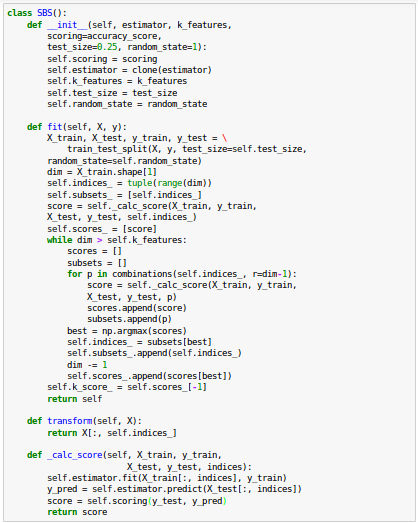
Now, it's time to see the SBS implementation in action using the KNN classifier from scikit-learn:

Our SBS implementation already splits the dataset into a test and training dataset inside the fit function, however, we still fed the training dataset X_train to the algorithm.
Then, the SBS fit method is going to create new training-subsets for testing (validation) and training, which is why this test set is also called validation dataset.
This approach is necessary to prevent our original test set becoming part of the training data.
Recall that our SBS algorithm collects the scores of the best feature subset at each stage, so let's move on to the more exciting part of our implementation and plot the classification accuracy of the KNN classifier that was calculated on the validation dataset:
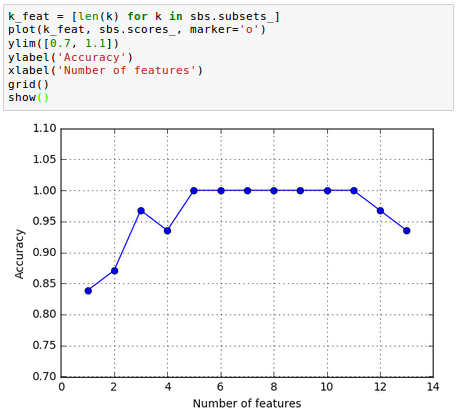
As we can see in the picture above, the accuracy of the KNN classifier improved on the validation dataset as we reduced the number of features, which is likely due to a decrease of the curse of dimensionality. Also note that the classifier achieved 100 percent accuracy for $k={5, 6, 7, 8, 9, 10}$:
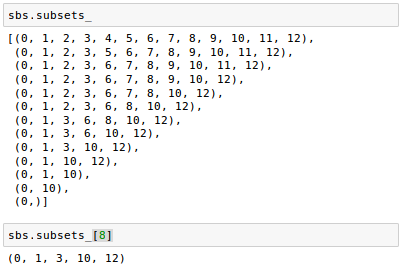
Let's see what those five features are that yielded such a good performance on the validation dataset:

Note that we obtained the column indices of the 5-feature subset from the 9 th position in the sbs.subsets_ attribute and returned the corresponding feature names from the column-index of the pandas Wine DataFrame:
Now we want to evaluate the performance of the KNN classifier on the original test set:

In the code, we used the complete feature set and obtained ~98.4 percent accuracy on the training dataset. However, the accuracy on the test dataset was slightly lower (~94.4 percent), which is an indicator of a slight degree of overfitting.
This time, let's use the selected 5-feature subset and see how well KNN performs:

Using fewer than half of the original features in the Wine dataset, the prediction accuracy on the test set improved by almost 2 percent. Also, we reduced overfitting, which we can tell from the small gap between test (~96.3 percent) and training (~96.0 percent) accuracy.
As an ensemble learning method for classification and regression, random forests or random decision forests operates by constructing a multitude of decision trees at training time and outputting the class (classification) or mean prediction (regression) of the individual trees.
In the previous sections, we used L1 regularization to remove irrelevant features via logistic regression and use the SBS algorithm for feature selection, the random forest is another approach to select relevant features from a dataset.
To select relevant features, unlike the L1 regularization case where we used our own algorithm for feature selection, the random forest implementation in scikit- learn already collects feature importances for us. So, all we have to do is to access them via the feature_importances_ attribute after fitting a RandomForestClassifier.
>Let's train a forest of 10,000 trees on the Wine dataset.
We're going to rank the 13 features by their respective importance measures.
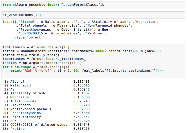
Here is the plot:
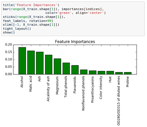
In the picture, the different features in the Wine dataset are ranked by their relative importance. Note that feature importances are normalized so that they sum up to 1.0.
From the plot we can see that the alcohol content of wine is the most discriminative feature in the dataset based on the average impurity decrease in the 10,000 decision trees.
"The random forest technique comes with an important gotcha that is worth mentioning. For instance, if two or more features are highly correlated, one feature may be ranked very highly while the information of the other feature(s) may not be fully captured. On the other hand, we don't need to be concerned about this problem if we are merely interested in the predictive performance of a model rather than the interpretation of feature importances." - Python Machine Learning by Sebastian Raschka
Source is available from bogotobogo-Machine-Learning .
Machine Learning with scikit-learn
scikit-learn installation
scikit-learn : Features and feature extraction - iris dataset
scikit-learn : Machine Learning Quick Preview
scikit-learn : Data Preprocessing I - Missing / Categorical data
scikit-learn : Data Preprocessing II - Partitioning a dataset / Feature scaling / Feature Selection / Regularization
scikit-learn : Data Preprocessing III - Dimensionality reduction vis Sequential feature selection / Assessing feature importance via random forests
Data Compression via Dimensionality Reduction I - Principal component analysis (PCA)
scikit-learn : Data Compression via Dimensionality Reduction II - Linear Discriminant Analysis (LDA)
scikit-learn : Data Compression via Dimensionality Reduction III - Nonlinear mappings via kernel principal component (KPCA) analysis
scikit-learn : Logistic Regression, Overfitting & regularization
scikit-learn : Supervised Learning & Unsupervised Learning - e.g. Unsupervised PCA dimensionality reduction with iris dataset
scikit-learn : Unsupervised_Learning - KMeans clustering with iris dataset
scikit-learn : Linearly Separable Data - Linear Model & (Gaussian) radial basis function kernel (RBF kernel)
scikit-learn : Decision Tree Learning I - Entropy, Gini, and Information Gain
scikit-learn : Decision Tree Learning II - Constructing the Decision Tree
scikit-learn : Random Decision Forests Classification
scikit-learn : Support Vector Machines (SVM)
scikit-learn : Support Vector Machines (SVM) II
Flask with Embedded Machine Learning I : Serializing with pickle and DB setup
Flask with Embedded Machine Learning II : Basic Flask App
Flask with Embedded Machine Learning III : Embedding Classifier
Flask with Embedded Machine Learning IV : Deploy
Flask with Embedded Machine Learning V : Updating the classifier
scikit-learn : Sample of a spam comment filter using SVM - classifying a good one or a bad one
Machine learning algorithms and concepts
Batch gradient descent algorithmSingle Layer Neural Network - Perceptron model on the Iris dataset using Heaviside step activation function
Batch gradient descent versus stochastic gradient descent
Single Layer Neural Network - Adaptive Linear Neuron using linear (identity) activation function with batch gradient descent method
Single Layer Neural Network : Adaptive Linear Neuron using linear (identity) activation function with stochastic gradient descent (SGD)
Logistic Regression
VC (Vapnik-Chervonenkis) Dimension and Shatter
Bias-variance tradeoff
Maximum Likelihood Estimation (MLE)
Neural Networks with backpropagation for XOR using one hidden layer
minHash
tf-idf weight
Natural Language Processing (NLP): Sentiment Analysis I (IMDb & bag-of-words)
Natural Language Processing (NLP): Sentiment Analysis II (tokenization, stemming, and stop words)
Natural Language Processing (NLP): Sentiment Analysis III (training & cross validation)
Natural Language Processing (NLP): Sentiment Analysis IV (out-of-core)
Locality-Sensitive Hashing (LSH) using Cosine Distance (Cosine Similarity)
Artificial Neural Networks (ANN)
[Note] Sources are available at Github - Jupyter notebook files1. Introduction
2. Forward Propagation
3. Gradient Descent
4. Backpropagation of Errors
5. Checking gradient
6. Training via BFGS
7. Overfitting & Regularization
8. Deep Learning I : Image Recognition (Image uploading)
9. Deep Learning II : Image Recognition (Image classification)
10 - Deep Learning III : Deep Learning III : Theano, TensorFlow, and Keras
Ph.D. / Golden Gate Ave, San Francisco / Seoul National Univ / Carnegie Mellon / UC Berkeley / DevOps / Deep Learning / Visualization