Machine Learning (Natural Language Processing - NLP) : Sentiment Analysis I

Sentiment analysis (opinion mining) is a subfield of natural language processing (NLP) and it is widely applied to reviews and social media ranging from marketing to customer service.

With this series of articles on sentiment analysis, we'll learn how to encode a document as a feature vector using the bag-of-words model. Then, we'll see how to weight the term frequency by relevance using term frequency-inverse document frequency.

Since working with a huge data can be quite expensive due to the large feature vectors that are created during this process, we'll also learn how to train a machine learning algorithm without loading the whole dataset into a computer's memory. We'll take out-of-core learning approach.

In this article, we will see how to use machine learning algorithms for classifying the attitude of a writer with regard to a particular topic or the overall contextual polarity of a document.

For our sentiment analysis, we will use a large dataset of movie reviews from the Internet Movie Database (IMDb) that has been collected by Maas et al. Learning Word Vectors for Sentiment Analysis. In the proceedings of the 49th Annual Meeting of the Association for Computational Linguistics: Human Language Technologies, pages 142-150, Portland, Oregon, USA, June 2011. Association for Computational Linguistics).

It has 50,000 polar movie reviews, and they are labeled as either positive or negative.

A movie was rated positive if it has more than six stars and a movie was rated negative if it has fewer than five stars on IMDb.

We can get the gz file:

$ wget http://ai.stanford.edu/~amaas/data/sentiment/aclImdb_v1.tar.gz
$ tar xvzf aclImdb_v1.tar.gz

The archive provids a set of 25,000 highly polar movie reviews for training, and 25,000 for testing. Also, it has additional unlabeled data as well.

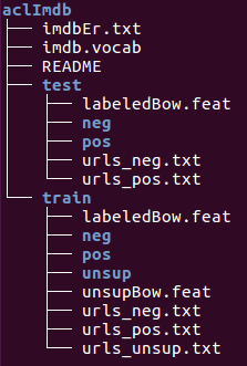
Now we want to assemble the individual text documents from the decompressed download archive into a single CSV file.

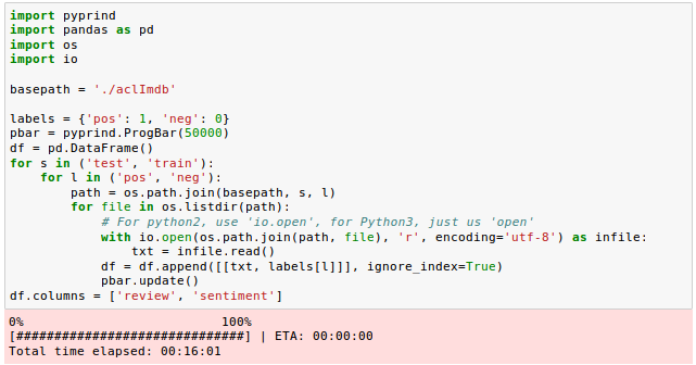
In the following code section, we will be reading the movie reviews into a pandas DataFrame object, and it may take a while (~10 minutes).

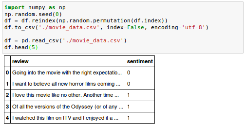
Let's see how our Dataframe looks like:

As we can see from the Jupyter notebook, we iterated over the train and test subdirectories in the main aclImdb directory and read the individual text files from the pos and neg subdirectories. We appended them to the DataFrame df with an integer class label (1 = positive and 0 = negative).

The class labels in the assembled dataset are sorted, so we may want to shuffle DataFrame using the permutation() function from the np.random submodule. This will be helpful to split the dataset into training and test sets in later sections when we stream the data from our local drive directly.
We may also want to store the assembled and shuffled movie review dataset as a CSV file:

The bag-of-words model is a simplifying representation used in natural language processing and information retrieval (IR). In this model, a text (such as a sentence or a document) is represented as the bag (multiset) of its words, disregarding grammar and even word order but keeping multiplicity - from wiki

The bag-of-words model allows us to represent text as numerical feature vectors. It is commonly used in methods of document classification where the (frequency of) occurrence of each word is used as a feature for training a classifier. It can be summarized as follows:

1. Create a vocabulary of unique tokens from the entire set of documents.
2. Construct a feature vector from each document that contains the counts of how often each word occurs in the particular document.

The feature vectors consist of mostly zeros and is called sparse since the unique words in each document represent only a small subset of all the words in the bag-of-words vocabulary.

We can use sklearn.feature_extraction.text.CountVectorizer to construct a bag-of-words model based on the word counts in the respective documents. It implements both tokenization and occurrence counting in a single class:

Let’s use it to tokenize and count the word occurrences with corpus of text documents:

The fit_transform method on CountVectorizer constructs the vocabulary of the bag-of-words model. The default configuration tokenizes the string by extracting words of at least 2 letters. The two sentences are transformed into sparse feature vectors:

Each index position in the feature vectors shown here corresponds to the integer values that are stored as dictionary items in the CountVectorizer vocabulary.

The words are stored in a Python dictionary, which maps the unique words that are mapped to integer indices:

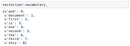
We have 9 vocabularies, 'and', 'document',..., 'this'.

The converse mapping from feature name to column index is stored in the vocabulary_ attribute of the vectorizer:

So, any words that were not seen in the training corpus will be completely ignored in future calls to the transform method:

ref: Feature extraction

When analyzing text data, there are words that occur across multiple documents. Those frequently occurring words typically don't contain useful or discriminatory information.

In other words, the frequent words such as "a", "the", and "is" carry very little meaningful information about the actual contents of the document.

In this section, we will learn about a useful transformation technique called term frequency-inverse document frequency (tf-idf). We'll use it to re-weight those frequently occurring words in the feature vectors. In order to re-weight the count features into floating point values suitable for usage by a classifier we need to use the tf-idf transform which can be defined as the product of the term frequency and the inverse document frequency:

where $\text{tf}$ means term-frequency while $\text{tf-idf}$ means term-frequency times inverse document-frequency.

The inverse document frequency $\text{idf}(t, d)$ can be defined as:

where $n_d$ is the total number of documents, and $\text{df}(d,t)$ is the number of documents $d$ that contain the term $t$.

Note that the $log$ is used to ensure that low document frequencies are not given too much weight.

Let's be more specific using the "corpus" document:

corpus = [
    'This is the first document.',
    'This is the second second.',
    'And the third one.',
    'Is this the first document?',
    ]

For the "is" term in the 4th document(d4). The term frequency $\text{tf}$ for "is" 1 since it appeared only once. The document frequency of this term ($\text{df(d,t)}$) is 3 since the term is occurs in three documents. The total number of document $n_d=4$, so we can calculate the $\text{idf}$ as follows:

TfidfTransformer() takes the raw term frequencies from CountVectorizer as input and transforms them into $ \text{tf-idfs}$:

Here, we used the "corpus" document of the example in the previous section.

Note that the frequent term such as "the" (index 6) that appeared in all document got lower $\text{tf-idf}$ (0.24 or 0.43) because it is unlikely to contain any useful and discriminatory information while "second" (index 5) got lower $\text{tf-idf}$ (0.86) because the term "second" appeared only in one document out of four documents.

The weights of each feature computed by the fit method call are stored in a model attribute:

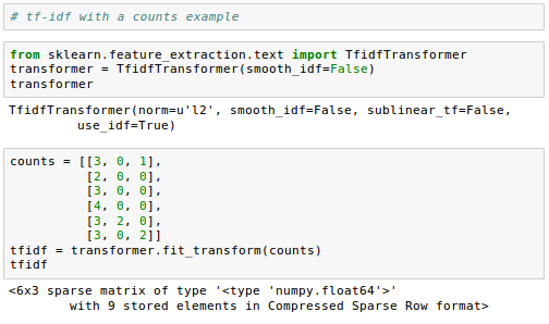
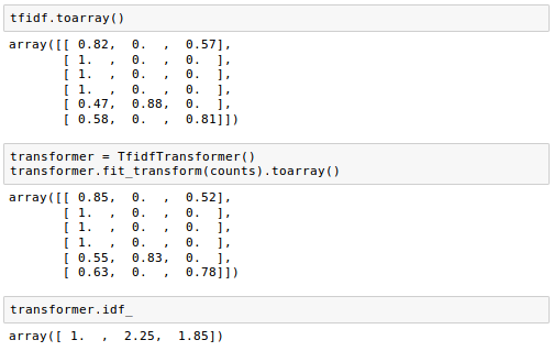
The following sample is from Feature extraction.

Github Jupyter notebook is available from Sentiment Analysis

Next: Machine Learning (Natural Language Processing - NLP): Sentiment Analysis II