Algorithms - Uniform Distribution of Points on the Surface of a Sphere
In this page, I'll try to distribute poinsts uniformly on the surface of a sphere. Though there are literally hundreds solutions out there, I'll take only one approach: random distribution.
I'll also show some cases:
- Directly working on a sphere using inverse CDF.
- Distribute points on a cylinder first, then map those points onto a sphere. (Archimedes' Theorem)
The following list is from TOPICS ON SPHERE DISTRIBUTIONS.
- What does it mean to place N points "evenly" on a sphere?
- Maximizes distances among neighboring points. However, the extreme values of D will be attained more than once. Also, there are several natural choices for the measures such as average distance or potential energy etc.
- Are there some values of N which are better than others?
- How can you describe locations on a sphere, anyway?
- Can you give a quick approximation to a good distribution?
- How can we improve an approximate solution?
- What if I want randomly to place points with a uniform distribution?
- Can this be generalized to higher-dimensional spheres?
- How is this related to collections of linear subspaces?
- Where can I get the coordinates of the vertices of the Platonic solids?
- How come this sounds like sphere packing?
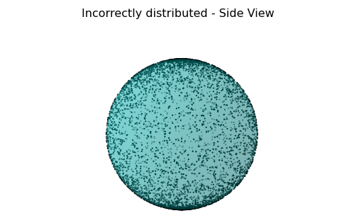
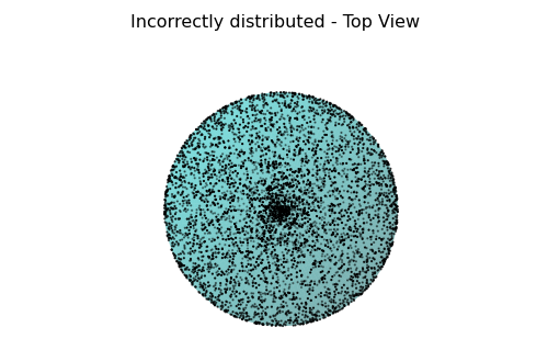
To distribute points uniformly on the surface of a sphere, it is tempting to use uniform distributions of $\phi$. But it's an incorrect choice as discussed in http://en.wikibooks.org/wiki/Mathematica/Uniform_Spherical_Distribution. That's because the area element $d\Omega(=\sin\phi d\theta d\phi)$ is a function of $\phi$, and the points selected in this way will be "bunched" near the poles (Sphere Point Picking).
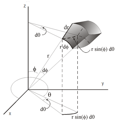
In Cartesian coordinates:
$$x=r\sin\phi\cos\theta$$
$$y=r\sin\phi\sin\theta$$
$$z=r\cos\phi$$
The differential solid is given by
$$d\Omega=\sin\phi d\theta d\phi$$
Archimedes' Theorem says axial projection of any measurable region on a sphere on the right circular cylinder circumscribed about the sphere preserves area.
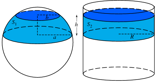
picture from Archimedes' Hat-Box Theorem.
Enclose a sphere in a cylinder and cut out a spherical segment by slicing perpendicularly to the cylinder's axis. Then the lateral surface area of the spherical segment $S1$ is equal to the lateral surface area cut out of the cylinder $S2$ by the same slicing planes.
$$S=S1=S2=2\pi Rh$$where $R$ is the radius of the cylinder (and tangent sphere) and $h$ is the height of the cylindrical (and spherical) segment.
So, this leads us to use Archimedes' theorem to distribute points on a sphere.
Generate a random point on the cylinder
$[- 1,1] \times [0,2\pi]$ and then find its inverse axial projection on the unit sphere. If a random point
is uniformly distributed on the cylinder, its inverse axial projection
will be uniformly distributed on the sphere.
As defined above, $\Omega$ is the solid angle. The probability that a point lies in an infinitesimal cone is $$P(\Omega)d\Omega$$ We get the following if we normalize $$\displaystyle \int_{\phi}\int_{\theta} P(\Omega)d\Omega = 1,$$ then, since the surface area of a sphere is $4\pi R^2$, the probability density function (PDF) for uniform density over a unit sphere becomes $$P(\Omega) = \frac{1}{4\pi}.$$
The probability can also be defined as below: $$P(\Omega)d\Omega= P(\theta,\phi) d\theta d\phi$$ where $\phi$ is the polar angle (aka zenith angle or colatitude) and $\theta$ is the azimuthal angle in $xy$-plane from $x$-axis. If we use $\displaystyle d\Omega = \sin\phi d\theta d\phi$, $$P(\Omega)d\Omega= P(\theta,\phi) d\theta d\phi$$ $$\frac{1}{4\pi}\sin\phi d\theta d\phi = P(\theta,\phi) d\theta d\phi$$ we get, $$P(\theta,\phi) = \frac{\sin\phi}{4\pi}.$$
Therefore, $$P(\phi) = \int_0^{2\pi}P(\theta,\phi)d\theta = \frac{\sin \phi}{2}$$ $$P(\theta) = \int_0^\pi P(\theta,\phi)d\phi = \frac{1}{2\pi}.$$
Now we just need to randomly generate $\phi$ and $\theta$ from their cumulative densities function (CDF), $F(\phi)$ and $F(\theta)$: $$F(\phi) = \int_0^\phi P(\phi) d\phi = \int_0^\phi \frac{\sin \phi}{2} d\phi = \frac{1- \cos \phi}{2}$$ $$F(\theta) = \int_0^\theta P(\theta) d\theta = \int_0^\theta \frac{1}{2\pi} d\theta = \frac{\theta}{2\pi}$$
To distribute points such that any small area on the sphere expected to contain same number of points, we choose two random variables $u,v$ which are uniform on the interval $[0,1]$. In other words, let $v = F(\phi)$ and $u = F(\theta)$ be independent uniform random
variables on $[0,1]$.
If we solve for $\theta$ and $\phi$, we get the following inverse functions of the CDFs
$$F^{-1}(v) = \phi = \cos^{-1}(2v-1)$$
$$F^{-1}(u) = \theta = 2\pi u.$$
Now we can use these to generate $x$, $y$ and $z$. Let's distribute the points uniformly on the surface of a sphere.
The followings sampling used random numbers. The incorrect ones used normal random numbers while the correct (at least better) ones reflected the dependency of $\phi$.
$$P(\phi) = \frac{\sin \phi}{2}$$In other words, by using inverse of CDF (Cumulative Distribution Function) defined in the previous section,
we get the correct random variable for $\phi = \cos^{-1}(2v-1)$ and $\theta = 2\pi u.$
In the calculation, the number of the sampling points were 5,000 and Matplotlib which utilizes NumPy were used for the plots. To draw pictures, we can just run the python script provided (see python script) after specifying the path for the data file generated from the calculation.
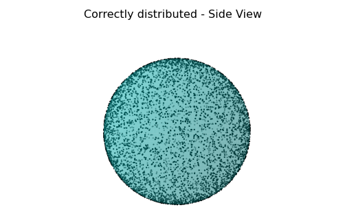
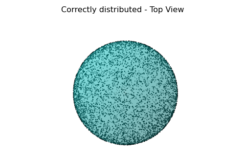
Here is the minimal C++ code. Revised codes are given in later section.
#include <iostream>
#include <fstream>
#include <ctime>
#include <cmath>
#include <vector>
using namespace std;

const double PI = 3.141592654;
const int nSample = 5000;
double irand(int min, int max);
int writeData(const vector<double>&x, const vector<double>&y, const vector<double>&z);

int main()
{
  srand( (unsigned)time( NULL ) );

  vector<double> x(nSample), y(nSample), z(nSample);

  double theta = 0, phi = 0;
  for(int i = 0; i < nSample; i++) {
    theta = 2*PI*irand(0,1);
    // corrrect
    phi = acos(2*irand(0,1)-1.0);
    // incorrect
    //phi = PI*irand(0,1);
    x[i] = cos(theta)*sin(phi);
    y[i] = sin(theta)*sin(phi);
    z[i] = cos(phi);
  }

  writeData(x, y, z);

  return 0;
}

// generate random number for the range (min, max)
double irand(int min, int max)
{
    return ((double)rand() / ((double)RAND_MAX + 1.0)) * (max - min) + min;
}

// write Cartesian coordinates (xyz)
int writeData(const vector<double>&x, const vector<double>&y, const vector<double>&z)
{
  ofstream ofs("sample.csv");

  if( ! ofs ) {
    cout << "Error opening file for output" << endl ;
    return -1 ;
  }

  for(int i = 0; i < nSample; i++) {
    ofs << x[i] << ',' << y[i]<< ',' << z[i]<< endl ;
  }

  ofs.close() ;
  return 0;
}
According to Archimedes' Theorem, when we project the surface of a cylinder to a sphere, the area preserved. So, we can distribute the points on the cylinder, then map those points onto a sphere. This is much easier approach that handling the solid angle ($\phi$) dependency.
The coding is less involved compared with the example shown previously. Other parts are the same, we just have to change some of the lines:
  for(int i = 0; i < nSample; i++) {
    theta = 2*PI*irand(0,1);
    z[i] = irand(0,1);
    x[i] = sqrt(1-z[i]*z[i])*cos(theta);
    y[i] = sqrt(1-z[i]*z[i])*sin(theta);
  }
$z$ stays the same for cylinder and sphere. The $\sqrt{1-z^2}$ is a radius at $z$ level after mapped onto a sphere. With that radius we can calculate $x$ and $y$. That's it!
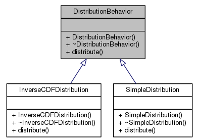
This code uses random approach, and using two methods:
- Simple distribution
simple distribution not considering the solid angle ($\phi$) effect. - Inverse CDF
This approach considers the Jacobian effect on the distribution
Here is the list of code, and can get them from KHong_Sample_Code.tar.gz.
Defaults.h
DistributionBehavior.cpp
DistributionBehavior.h
InverseCDFDistribution.cpp
InverseCDFDistribution.h
Main.cpp
Makefile
MethodCollection.cpp
MethodCollection.h
MyRandom.cpp
MyRandom.h
Points.cpp
Points.h
README
Sampling.cpp
Sampling.h
SimpleDistribution.cpp
SimpleDistribution.h
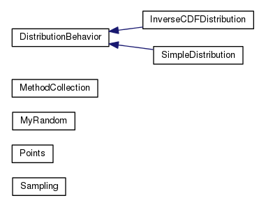
Get more information from Doxygen.
Here is one of the class diagrams that can be found in the Doxygen:

Ph.D. / Golden Gate Ave, San Francisco / Seoul National Univ / Carnegie Mellon / UC Berkeley / DevOps / Deep Learning / Visualization