Artificial Neural Network (ANN) 9 - Deep Learning II : Image Recognition (Image Classification)
Continued from Deep Learning I : Image Recognition (Image uploading).
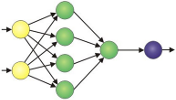
In this section, we will now implement the code with one hidden, and one output layer to classify the MNIST images:
import numpy as np
from scipy.special import expit
import sys


class NeuralNetMLP(object):
    """ Feedforward neural network / Multi-layer perceptron classifier.

    Parameters
    ------------
    n_output : int
        Number of output units, should be equal to the
        number of unique class labels.
    n_features : int
        Number of features (dimensions) in the target dataset.
        Should be equal to the number of columns in the X array.
    n_hidden : int (default: 30)
        Number of hidden units.
    l1 : float (default: 0.0)
        Lambda value for L1-regularization.
        No regularization if l1=0.0 (default)
    l2 : float (default: 0.0)
        Lambda value for L2-regularization.
        No regularization if l2=0.0 (default)
    epochs : int (default: 500)
        Number of passes over the training set.
    eta : float (default: 0.001)
        Learning rate.
    alpha : float (default: 0.0)
        Momentum constant. Factor multiplied with the
        gradient of the previous epoch t-1 to improve
        learning speed
        w(t) := w(t) - (grad(t) + alpha*grad(t-1))
    decrease_const : float (default: 0.0)
        Decrease constant. Shrinks the learning rate
        after each epoch via eta / (1 + epoch*decrease_const)
    shuffle : bool (default: True)
        Shuffles training data every epoch if True to prevent circles.
    minibatches : int (default: 1)
        Divides training data into k minibatches for efficiency.
        Normal gradient descent learning if k=1 (default).
    random_state : int (default: None)
        Set random state for shuffling and initializing the weights.

    Attributes
    -----------
    cost_ : list
      Sum of squared errors after each epoch.

    """
    def __init__(self, n_output, n_features, n_hidden=30,
                 l1=0.0, l2=0.0, epochs=500, eta=0.001,
                 alpha=0.0, decrease_const=0.0, shuffle=True,
                 minibatches=1, random_state=None):

        np.random.seed(random_state)
        self.n_output = n_output
        self.n_features = n_features
        self.n_hidden = n_hidden
        self.w1, self.w2 = self._initialize_weights()
        self.l1 = l1
        self.l2 = l2
        self.epochs = epochs
        self.eta = eta
        self.alpha = alpha
        self.decrease_const = decrease_const
        self.shuffle = shuffle
        self.minibatches = minibatches

    def _encode_labels(self, y, k):
        """Encode labels into one-hot representation

        Parameters
        ------------
        y : array, shape = [n_samples]
            Target values.

        Returns
        -----------
        onehot : array, shape = (n_labels, n_samples)

        """
        onehot = np.zeros((k, y.shape[0]))
        for idx, val in enumerate(y):
            onehot[val, idx] = 1.0
        return onehot

    def _initialize_weights(self):
        """Initialize weights with small random numbers."""
        w1 = np.random.uniform(-1.0, 1.0,
                               size=self.n_hidden*(self.n_features + 1))
        w1 = w1.reshape(self.n_hidden, self.n_features + 1)
        w2 = np.random.uniform(-1.0, 1.0,
                               size=self.n_output*(self.n_hidden + 1))
        w2 = w2.reshape(self.n_output, self.n_hidden + 1)
        return w1, w2

    def _sigmoid(self, z):
        """Compute logistic function (sigmoid)

        Uses scipy.special.expit to avoid overflow
        error for very small input values z.

        """
        # return 1.0 / (1.0 + np.exp(-z))
        return expit(z)

    def _sigmoid_gradient(self, z):
        """Compute gradient of the logistic function"""
        sg = self._sigmoid(z)
        return sg * (1.0 - sg)

    def _add_bias_unit(self, X, how='column'):
        """Add bias unit (column or row of 1s) to array at index 0"""
        if how == 'column':
            X_new = np.ones((X.shape[0], X.shape[1] + 1))
            X_new[:, 1:] = X
        elif how == 'row':
            X_new = np.ones((X.shape[0] + 1, X.shape[1]))
            X_new[1:, :] = X
        else:
            raise AttributeError('`how` must be `column` or `row`')
        return X_new

    def _feedforward(self, X, w1, w2):
        """Compute feedforward step

        Parameters
        -----------
        X : array, shape = [n_samples, n_features]
            Input layer with original features.
        w1 : array, shape = [n_hidden_units, n_features]
            Weight matrix for input layer -> hidden layer.
        w2 : array, shape = [n_output_units, n_hidden_units]
            Weight matrix for hidden layer -> output layer.

        Returns
        ----------
        a1 : array, shape = [n_samples, n_features+1]
            Input values with bias unit.
        z2 : array, shape = [n_hidden, n_samples]
            Net input of hidden layer.
        a2 : array, shape = [n_hidden+1, n_samples]
            Activation of hidden layer.
        z3 : array, shape = [n_output_units, n_samples]
            Net input of output layer.
        a3 : array, shape = [n_output_units, n_samples]
            Activation of output layer.

        """
        a1 = self._add_bias_unit(X, how='column')
        z2 = w1.dot(a1.T)
        a2 = self._sigmoid(z2)
        a2 = self._add_bias_unit(a2, how='row')
        z3 = w2.dot(a2)
        a3 = self._sigmoid(z3)
        return a1, z2, a2, z3, a3

    def _L2_reg(self, lambda_, w1, w2):
        """Compute L2-regularization cost"""
        return (lambda_/2.0) * (np.sum(w1[:, 1:] ** 2) +
                                np.sum(w2[:, 1:] ** 2))

    def _L1_reg(self, lambda_, w1, w2):
        """Compute L1-regularization cost"""
        return (lambda_/2.0) * (np.abs(w1[:, 1:]).sum() +
                                np.abs(w2[:, 1:]).sum())

    def _get_cost(self, y_enc, output, w1, w2):
        """Compute cost function.

        Parameters
        ----------
        y_enc : array, shape = (n_labels, n_samples)
            one-hot encoded class labels.
        output : array, shape = [n_output_units, n_samples]
            Activation of the output layer (feedforward)
        w1 : array, shape = [n_hidden_units, n_features]
            Weight matrix for input layer -> hidden layer.
        w2 : array, shape = [n_output_units, n_hidden_units]
            Weight matrix for hidden layer -> output layer.

        Returns
        ---------
        cost : float
            Regularized cost.

        """
        term1 = -y_enc * (np.log(output))
        term2 = (1.0 - y_enc) * np.log(1.0 - output)
        cost = np.sum(term1 - term2)
        L1_term = self._L1_reg(self.l1, w1, w2)
        L2_term = self._L2_reg(self.l2, w1, w2)
        cost = cost + L1_term + L2_term
        return cost

    def _get_gradient(self, a1, a2, a3, z2, y_enc, w1, w2):
        """ Compute gradient step using backpropagation.

        Parameters
        ------------
        a1 : array, shape = [n_samples, n_features+1]
            Input values with bias unit.
        a2 : array, shape = [n_hidden+1, n_samples]
            Activation of hidden layer.
        a3 : array, shape = [n_output_units, n_samples]
            Activation of output layer.
        z2 : array, shape = [n_hidden, n_samples]
            Net input of hidden layer.
        y_enc : array, shape = (n_labels, n_samples)
            one-hot encoded class labels.
        w1 : array, shape = [n_hidden_units, n_features]
            Weight matrix for input layer -> hidden layer.
        w2 : array, shape = [n_output_units, n_hidden_units]
            Weight matrix for hidden layer -> output layer.

        Returns
        ---------
        grad1 : array, shape = [n_hidden_units, n_features]
            Gradient of the weight matrix w1.
        grad2 : array, shape = [n_output_units, n_hidden_units]
            Gradient of the weight matrix w2.

        """
        # backpropagation
        sigma3 = a3 - y_enc
        z2 = self._add_bias_unit(z2, how='row')
        sigma2 = w2.T.dot(sigma3) * self._sigmoid_gradient(z2)
        sigma2 = sigma2[1:, :]
        grad1 = sigma2.dot(a1)
        grad2 = sigma3.dot(a2.T)

        # regularize
        grad1[:, 1:] += self.l2 * w1[:, 1:]
        grad1[:, 1:] += self.l1 * np.sign(w1[:, 1:])
        grad2[:, 1:] += self.l2 * w2[:, 1:]
        grad2[:, 1:] += self.l1 * np.sign(w2[:, 1:])

        return grad1, grad2

    def predict(self, X):
        """Predict class labels

        Parameters
        -----------
        X : array, shape = [n_samples, n_features]
            Input layer with original features.

        Returns:
        ----------
        y_pred : array, shape = [n_samples]
            Predicted class labels.

        """
        if len(X.shape) != 2:
            raise AttributeError('X must be a [n_samples, n_features] array.\n'
                                 'Use X[:,None] for 1-feature classification,'
                                 '\nor X[[i]] for 1-sample classification')

        a1, z2, a2, z3, a3 = self._feedforward(X, self.w1, self.w2)
        y_pred = np.argmax(z3, axis=0)
        return y_pred

    def fit(self, X, y, print_progress=False):
        """ Learn weights from training data.

        Parameters
        -----------
        X : array, shape = [n_samples, n_features]
            Input layer with original features.
        y : array, shape = [n_samples]
            Target class labels.
        print_progress : bool (default: False)
            Prints progress as the number of epochs
            to stderr.

        Returns:
        ----------
        self

        """
        self.cost_ = []
        X_data, y_data = X.copy(), y.copy()
        y_enc = self._encode_labels(y, self.n_output)

        delta_w1_prev = np.zeros(self.w1.shape)
        delta_w2_prev = np.zeros(self.w2.shape)

        for i in range(self.epochs):

            # adaptive learning rate
            self.eta /= (1 + self.decrease_const*i)

            if print_progress:
                sys.stderr.write('\rEpoch: %d/%d' % (i+1, self.epochs))
                sys.stderr.flush()

            if self.shuffle:
                idx = np.random.permutation(y_data.shape[0])
                X_data, y_enc = X_data[idx], y_enc[:, idx]

            mini = np.array_split(range(y_data.shape[0]), self.minibatches)
            for idx in mini:

                # feedforward
                a1, z2, a2, z3, a3 = self._feedforward(X_data[idx],
                                                       self.w1,
                                                       self.w2)
                cost = self._get_cost(y_enc=y_enc[:, idx],
                                      output=a3,
                                      w1=self.w1,
                                      w2=self.w2)
                self.cost_.append(cost)

                # compute gradient via backpropagation
                grad1, grad2 = self._get_gradient(a1=a1, a2=a2,
                                                  a3=a3, z2=z2,
                                                  y_enc=y_enc[:, idx],
                                                  w1=self.w1,
                                                  w2=self.w2)

                delta_w1, delta_w2 = self.eta * grad1, self.eta * grad2
                self.w1 -= (delta_w1 + (self.alpha * delta_w1_prev))
                self.w2 -= (delta_w2 + (self.alpha * delta_w2_prev))
                delta_w1_prev, delta_w2_prev = delta_w1, delta_w2

        return self
Here is the summary of the parameters used in the code:
- l2 : The $\lambda$ parameter for L2 regularization to decrease the degree of overfitting; equivalently, $l1$ is the $\lambda$ parameter for L1 regularization.
- epochs : The number of passes over the training set. eta : The learning rate $\eta$.
- alpha : A parameter for momentum learning to add a factor of the previous gradient to the weight update for faster learning $\Delta \mathbf w_t = \eta \nabla J (\mathbf w_t) + \alpha \Delta \mathbf w_{t-1}$ (where $t$ is the current time step or epoch).
- decrease_const : The decrease constant $d$ for an adaptive learning rate $\eta$ that decreases over time for better convergence $\frac{\eta}{1 + t \times d}$.
- shuffle : Shuffling the training set prior to every epoch to prevent the algorithm from getting stuck in cycles.
- Minibatches : Splitting of the training data into SkS mini-batches in each epoch. The gradient is computed for each mini-batch separately instead of the entire training data for faster learning.
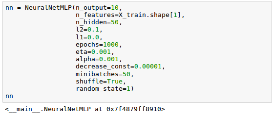
Let's initialize our neural network with 784 input units (n_features), 50 hidden units (n_hidden), and 10 output units (n_output):
Now it's time to train our neural network using 60,000 samples from the already shuffled MNIST training dataset. It may take a while:

We can now visualize the convergence of the cost function which is saved in a cost_ list. Note that we only plot every 50th step since we used the parameter minibatches=50, 50 mini-batches x 1000 epochs.
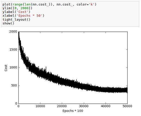
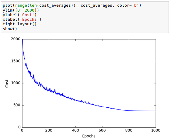
As we see in the plot above, while though the optimization algorithm converged around 800 epochs (40,000/50 = 800), the graph of the cost function looks very noisy. That's because we trained our neural network with mini-batch learning which computes the gradient using batch of 50 samples from dataset rather one sample at a time.
Note that the stochastic gradient descent (SGD) computes the gradient using a single sample while most applications of SGD actually use a minibatch of several samples.
We can make the noisy plot smoother by averaging over the mini-batch intervals:
We can evaluate the performance of the model by calculating the prediction accuracy:

Though we can see the model classifies most of the training digits correctly, let's see how does the model perform on the 10,000 test images:

Considering the small discrepancy between the two outputs, training and test dataset, we can see our model performs pretty well.
In order to further fine-tune our model, we may want to tweak the followings:
- the number of hidden units
- values of the regularization parameters
- learning rate
- the values of the decrease constant.
To make our model better, we need to know what image samples our model struggles with. Here are the samples that our model misclassified:
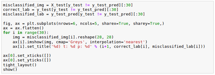
The picture below is the samples (6 x 5) that our model misclassifed. The 't' stands for the true class label while 'p' stands for the predicted class label:
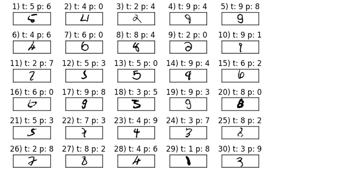
Considering some of those images are even challenging for us humans to classify correctly, our model did perform relatively well!
Python Machine Learning by Sebastian Raschka
part8-9-ImageRecognition.ipynb
10 - Deep Learning III : Deep Learning III : Theano, TensorFlow, and Keras
Machine Learning with scikit-learn
scikit-learn installation
scikit-learn : Features and feature extraction - iris dataset
scikit-learn : Machine Learning Quick Preview
scikit-learn : Data Preprocessing I - Missing / Categorical data
scikit-learn : Data Preprocessing II - Partitioning a dataset / Feature scaling / Feature Selection / Regularization
scikit-learn : Data Preprocessing III - Dimensionality reduction vis Sequential feature selection / Assessing feature importance via random forests
Data Compression via Dimensionality Reduction I - Principal component analysis (PCA)
scikit-learn : Data Compression via Dimensionality Reduction II - Linear Discriminant Analysis (LDA)
scikit-learn : Data Compression via Dimensionality Reduction III - Nonlinear mappings via kernel principal component (KPCA) analysis
scikit-learn : Logistic Regression, Overfitting & regularization
scikit-learn : Supervised Learning & Unsupervised Learning - e.g. Unsupervised PCA dimensionality reduction with iris dataset
scikit-learn : Unsupervised_Learning - KMeans clustering with iris dataset
scikit-learn : Linearly Separable Data - Linear Model & (Gaussian) radial basis function kernel (RBF kernel)
scikit-learn : Decision Tree Learning I - Entropy, Gini, and Information Gain
scikit-learn : Decision Tree Learning II - Constructing the Decision Tree
scikit-learn : Random Decision Forests Classification
scikit-learn : Support Vector Machines (SVM)
scikit-learn : Support Vector Machines (SVM) II
Flask with Embedded Machine Learning I : Serializing with pickle and DB setup
Flask with Embedded Machine Learning II : Basic Flask App
Flask with Embedded Machine Learning III : Embedding Classifier
Flask with Embedded Machine Learning IV : Deploy
Flask with Embedded Machine Learning V : Updating the classifier
scikit-learn : Sample of a spam comment filter using SVM - classifying a good one or a bad one
Machine learning algorithms and concepts
Batch gradient descent algorithmSingle Layer Neural Network - Perceptron model on the Iris dataset using Heaviside step activation function
Batch gradient descent versus stochastic gradient descent
Single Layer Neural Network - Adaptive Linear Neuron using linear (identity) activation function with batch gradient descent method
Single Layer Neural Network : Adaptive Linear Neuron using linear (identity) activation function with stochastic gradient descent (SGD)
Logistic Regression
VC (Vapnik-Chervonenkis) Dimension and Shatter
Bias-variance tradeoff
Maximum Likelihood Estimation (MLE)
Neural Networks with backpropagation for XOR using one hidden layer
minHash
tf-idf weight
Natural Language Processing (NLP): Sentiment Analysis I (IMDb & bag-of-words)
Natural Language Processing (NLP): Sentiment Analysis II (tokenization, stemming, and stop words)
Natural Language Processing (NLP): Sentiment Analysis III (training & cross validation)
Natural Language Processing (NLP): Sentiment Analysis IV (out-of-core)
Locality-Sensitive Hashing (LSH) using Cosine Distance (Cosine Similarity)
Artificial Neural Networks (ANN)
[Note] Sources are available at Github - Jupyter notebook files1. Introduction
2. Forward Propagation
3. Gradient Descent
4. Backpropagation of Errors
5. Checking gradient
6. Training via BFGS
7. Overfitting & Regularization
8. Deep Learning I : Image Recognition (Image uploading)
9. Deep Learning II : Image Recognition (Image classification)
10 - Deep Learning III : Deep Learning III : Theano, TensorFlow, and Keras
Ph.D. / Golden Gate Ave, San Francisco / Seoul National Univ / Carnegie Mellon / UC Berkeley / DevOps / Deep Learning / Visualization