scikit-learn : k-Nearest Neighbors (k-NN) Algorithm

k-Nearest Neighbor (k-NN) classifier is a supervised learning algorithm, and it is a lazy learner. It is called lazy algorithm because it doesn't learn a discriminative function from the training data but memorizes the training dataset instead.
The K-nearest neighbor classifier offers an alternative approach to classification using lazy learning that allows us to make predictions without any model training but at the cost of expensive prediction step.

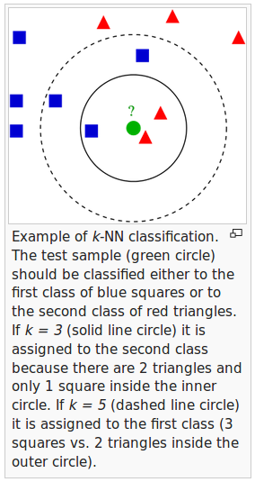
picture source - wiki
As shown in the description of the above picture, the k-NN algorithm can be summarized as following steps:
- Choose the number of $k$ and a distance metric.
- Find the $k$ nearest neighbors of the sample that we want to classify.
- Assign the class label by majority vote.
Pros and cons:
- Advantages:
k-NN is a memory-based approach is that the classifier immediately adapts as we collect new training data. - Downside:
The computational complexity for classifying new samples grows linearly with the number of samples in the training dataset in the worst-case scenario.
Note that we can't discard training samples since no training step is involved. Therefore, storage space can be challenging if we work with large datasets.
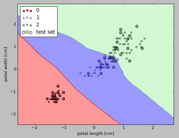
Here is the output from a k-NN model in scikit-learn using an Euclidean distance metric. With 5 neighbors in the KNN model for this dataset, we obtain a relatively smooth decision boundary:

The implemented code looks like this:
from sklearn import datasets
from sklearn.cross_validation import train_test_split

from sklearn.preprocessing import StandardScaler
from sklearn.neighbors import KNeighborsClassifier

import numpy as np
import matplotlib.pyplot as plt
from matplotlib.colors import ListedColormap

def plot_decision_regions(X, y, classifier, test_idx=None, resolution=0.02):
   # setup marker generator and color map
   markers = ('s', 'x', 'o', '^', 'v')
   colors = ('red', 'blue', 'lightgreen', 'gray', 'cyan')
   cmap = ListedColormap(colors[:len(np.unique(y))])

   # plot the decision surface
   x1_min, x1_max = X[:, 0].min() - 1, X[:, 0].max() + 1
   x2_min, x2_max = X[:, 1].min() - 1, X[:, 1].max() + 1
   xx1, xx2 = np.meshgrid(np.arange(x1_min, x1_max, resolution),
   np.arange(x2_min, x2_max, resolution))
   Z = classifier.predict(np.array([xx1.ravel(), xx2.ravel()]).T)
   Z = Z.reshape(xx1.shape)
   plt.contourf(xx1, xx2, Z, alpha=0.4, cmap=cmap)
   plt.xlim(xx1.min(), xx1.max())
   plt.ylim(xx2.min(), xx2.max())

   # plot all samples
   X_test, y_test = X[test_idx, :], y[test_idx]
   for idx, cl in enumerate(np.unique(y)):
      plt.scatter(x=X[y == cl, 0], y=X[y == cl, 1],
               alpha=0.8, c=cmap(idx),
               marker=markers[idx], label=cl)
   # highlight test samples
   if test_idx:
      X_test, y_test = X[test_idx, :], y[test_idx]
      plt.scatter(X_test[:, 0], X_test[:, 1], c='',
               alpha=1.0, linewidth=1, marker='o',
               s=55, label='test set')

iris = datasets.load_iris()
X = iris.data[:, [2, 3]]
y = iris.target

X_train, X_test, y_train, y_test = train_test_split(X, y, test_size=0.3, random_state=0)

sc = StandardScaler()
X_train_std = sc.fit_transform(X_train)
X_test_std = sc.fit_transform(X_test)

X_combined_std = np.vstack((X_train_std, X_test_std))
y_combined = np.hstack((y_train, y_test))

knn = KNeighborsClassifier(n_neighbors=5, p=2,
                           metric='minkowski')
knn.fit(X_train_std, y_train)

plot_decision_regions(X_combined_std, y_combined,
                      classifier=knn, test_idx=range(105,150))

plt.xlabel('petal length [cm]')
plt.ylabel('petal width [cm]')
plt.legend(loc='upper left')
plt.show()
The value of $k$ is crucial to find a good balance between over/under-fitting.
The distance metric should be appropriate for the features in the dataset. For a simple Euclidean distance metric is used for real-valued samples, for example, the flowers in our Iris dataset, which have features measured in centimeters.
However, if we are using a Euclidean distance measure, it is also important to standardize the data so that each feature contributes equally to the distance.
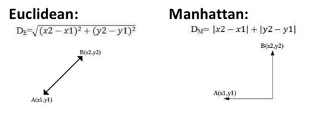
The 'minkowski' distance that we used in the code is just a generalization of the Euclidean and Manhattan distance:

The k-NN is very susceptible to overfitting due to the curse of dimensionality.
The curse of dimensionality happens when the feature space becomes increasingly sparse for an increasing number of dimensions of a fixed-size training dataset.
Basically, in a high-dimensional space, even the closest neighbors can be too far away to give a good estimate.
In that case, we use feature selection and dimensionality reduction techniques to avoid the curse of dimensionality.
To make good predictions we need to have informative and discriminatory features.
So, in subsequent articles, we will further discuss the preprocessing of data, dimensionality reduction, and feature selection to build a good machine learning models.
Data pre-processing is an important step in the data mining process. The phrase "garbage in, garbage out" is particularly applicable to data mining and machine learning projects. - https://en.wikipedia.org/wiki/Data_pre-processing
In machine learning and statistics, dimensionality reduction or dimension reduction is the process of reducing the number of random variables under consideration, via obtaining a set of principal variables. It can be divided into feature selection and feature extraction. - https://en.wikipedia.org/wiki/Dimensionality_reduction
Ref: Python Machine Learing by Sebastian Raschka
Machine Learning with scikit-learn
scikit-learn installation
scikit-learn : Features and feature extraction - iris dataset
scikit-learn : Machine Learning Quick Preview
scikit-learn : Data Preprocessing I - Missing / Categorical data
scikit-learn : Data Preprocessing II - Partitioning a dataset / Feature scaling / Feature Selection / Regularization
scikit-learn : Data Preprocessing III - Dimensionality reduction vis Sequential feature selection / Assessing feature importance via random forests
Data Compression via Dimensionality Reduction I - Principal component analysis (PCA)
scikit-learn : Data Compression via Dimensionality Reduction II - Linear Discriminant Analysis (LDA)
scikit-learn : Data Compression via Dimensionality Reduction III - Nonlinear mappings via kernel principal component (KPCA) analysis
scikit-learn : Logistic Regression, Overfitting & regularization
scikit-learn : Supervised Learning & Unsupervised Learning - e.g. Unsupervised PCA dimensionality reduction with iris dataset
scikit-learn : Unsupervised_Learning - KMeans clustering with iris dataset
scikit-learn : Linearly Separable Data - Linear Model & (Gaussian) radial basis function kernel (RBF kernel)
scikit-learn : Decision Tree Learning I - Entropy, Gini, and Information Gain
scikit-learn : Decision Tree Learning II - Constructing the Decision Tree
scikit-learn : Random Decision Forests Classification
scikit-learn : Support Vector Machines (SVM)
scikit-learn : Support Vector Machines (SVM) II
Flask with Embedded Machine Learning I : Serializing with pickle and DB setup
Flask with Embedded Machine Learning II : Basic Flask App
Flask with Embedded Machine Learning III : Embedding Classifier
Flask with Embedded Machine Learning IV : Deploy
Flask with Embedded Machine Learning V : Updating the classifier
scikit-learn : Sample of a spam comment filter using SVM - classifying a good one or a bad one
Machine learning algorithms and concepts
Batch gradient descent algorithmSingle Layer Neural Network - Perceptron model on the Iris dataset using Heaviside step activation function
Batch gradient descent versus stochastic gradient descent
Single Layer Neural Network - Adaptive Linear Neuron using linear (identity) activation function with batch gradient descent method
Single Layer Neural Network : Adaptive Linear Neuron using linear (identity) activation function with stochastic gradient descent (SGD)
Logistic Regression
VC (Vapnik-Chervonenkis) Dimension and Shatter
Bias-variance tradeoff
Maximum Likelihood Estimation (MLE)
Neural Networks with backpropagation for XOR using one hidden layer
minHash
tf-idf weight
Natural Language Processing (NLP): Sentiment Analysis I (IMDb & bag-of-words)
Natural Language Processing (NLP): Sentiment Analysis II (tokenization, stemming, and stop words)
Natural Language Processing (NLP): Sentiment Analysis III (training & cross validation)
Natural Language Processing (NLP): Sentiment Analysis IV (out-of-core)
Locality-Sensitive Hashing (LSH) using Cosine Distance (Cosine Similarity)
Artificial Neural Networks (ANN)
[Note] Sources are available at Github - Jupyter notebook files1. Introduction
2. Forward Propagation
3. Gradient Descent
4. Backpropagation of Errors
5. Checking gradient
6. Training via BFGS
7. Overfitting & Regularization
8. Deep Learning I : Image Recognition (Image uploading)
9. Deep Learning II : Image Recognition (Image classification)
10 - Deep Learning III : Deep Learning III : Theano, TensorFlow, and Keras
Ph.D. / Golden Gate Ave, San Francisco / Seoul National Univ / Carnegie Mellon / UC Berkeley / DevOps / Deep Learning / Visualization