Artificial Neural Network (ANN) 3 - Gradient Descent

bogotobogo.com site search:

Note

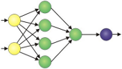
Continued from Artificial Neural Network (ANN) 2 - Forward Propagation where we built a neural network.

However, it gave us quite terrible predictions of our score on a test based on how many hours we slept and how many hours we studied the night before.

In this article, we'll focus on the theory of making those predictions better.

Here are the equations for each layer and the diagram:

$$ \begin{align}z^{(2)} = XW^{(1)} \tag 1\\ a^{(2)} = f \left( z^{(2)} \right)& \tag 2\\ z^{(3)} = a^{(2)} W^{(2)} \tag 3\\ \hat y = f \left( z^{(3)} \right) \tag 4 \end{align} $$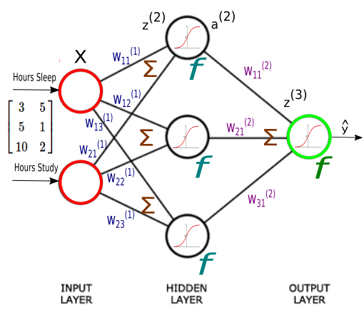

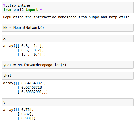
$\hat y$ and $y$

Here are the values of $\hat y$ and $y$:

Plot looks like this:

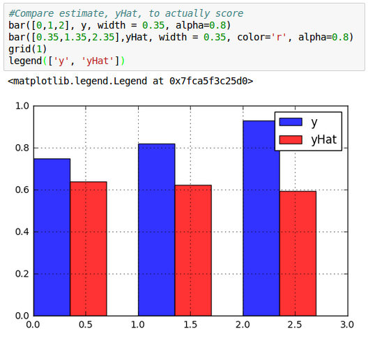
We can see our predictions ($\hat y$) are pretty inaccurate!

Cost function $J$

To improve our poor model, we first need to find a way of quantifying exactly how wrong our predictions are.

One way of doing it is to use a cost function. For a given sample, a cost function tells us how costly our models is.

We'll use sum of square errors to compute an overall cost and we'll try to minimize it. Actually, training a network means minimizing a cost function.

$$ J = \sum_{i=1}^N (y_i-\hat y_i) $$

where the $N$ is the number of training samples.

As we can see from equation, the cost is a function of two things: our sample data and the weights on our synapses. Since we don't have much control of our data, we'll try to minimize our cost by changing the weights.

We have a collection of 9 weights:

$$ W^{(1)} = \begin{bmatrix} W_{11}^{(1)} & W_{12}^{(1)} & W_{13}^{(1)} \\ W_{21}^{(1)} & W_{22}^{(1)} & W_{23}^{(1)} \end{bmatrix} $$ $$ W^{(2)} = \begin{bmatrix} W_{11}^{(2)} \\ W_{21}^{(2)} \\ W_{31}^{(2)} \end{bmatrix} $$

and we're going to make our cost ($J$) as small as possible with a optimal combination of the weights.

Curse of dimensionality

Well, we're not there yet. Considering the 9 weights, finding the right combination that gives us minimum $J$ may be costly.

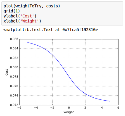
Let's try the case when we tweek only one weight value ($W_{11}^{(1)}) in the range [-5,5] with 1000 try. Other weights remain untouched with the values of randomly initialized in "__init__()" method:

Here is the code for the 1-weight:

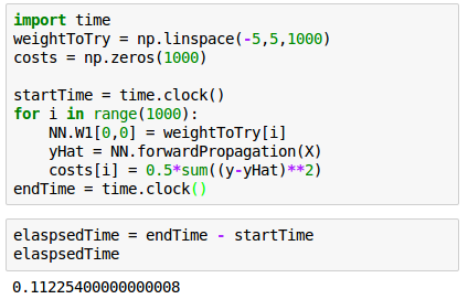
It takes about 0.11 seconds to check 1000 different weight values for our neural network. Since we've computed the cost for a wide range values of $W$, we can just pick the one with the smallest cost, let that be our weight, and we've trained our network.

Here is the plot for the 1000 weights:

Note that we have 9! But this time, let's do just 2 weights. To maintain the same precision we now need to check 1000 times 1000, or one million values:

For 1 million evaluations, it took an 100 seconds! The real curse of dimensionality kicks in as we continue to add dimensions. Searching through three weights would take a billion evaluations, 100*1000 sec = 27 hrs!

For our all 9 weights, it could take "1,268,391,679,350", 1 trillion millenium!:

Gradient descent method

So, we may want to use gradient descent algorithm to get the weights that take $J$ to minimum. Though it may not seem so impressive in one dimension, it is capable of incredible speedups in higher dimensions.

Actually, I wrote couple of articles on gradient descent algorithm:

Though we have two choices of the gradient descent: batch(standard) or stochastic, we're going to use the batch to train our Neural Network.

In batch gradient descent method sums up all the derivatives of $J$ for all samples:

$$ \sum \frac {\partial J}{\partial W} $$ while the stochastic gradient descent (SGD) method uses one derivative at one sample and move to another sample point:

$$ \frac {\partial J}{\partial W} $$

Next:

4. Backpropagation