Artificial Neural Network (ANN) 6 - Training via BFGS
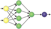
Continued from Artificial Neural Network (ANN) 5 - Checking gradient where computed the gradient of our cost function and check the computing accuracy and added helper function to our neural network class so that we are ready to train our Neural Network.
In this article, we're going to use a variant of gradient descent method known as Broyden-Fletcher-Goldfarb-Shanno (BFGS) optimization algorithm.
The BFGS algorithm overcomes some of the limitations of plain gradient descent by seeking the second derivative (a stationary point) of the cost function.
For such problems, a necessary condition for optimality is that the gradient be zero. Newton's method and the BFGS methods are not guaranteed to converge unless the function has a quadratic Taylor expansion near an optimum. These methods use both the first and second derivatives of the function. However, BFGS has proven to have good performance even for non-smooth optimizations. - wiki - Broyden-Fletcher-Goldfarb-Shanno algorithm
Once the network is trained, we'll use trained parameters instead of random parameters.
However, we're not going to write the BFGS algorithm but we'll use scipy's optimize package (scipy.optimize.minimize) instead.
Here is a code defining a "Trainer" class:
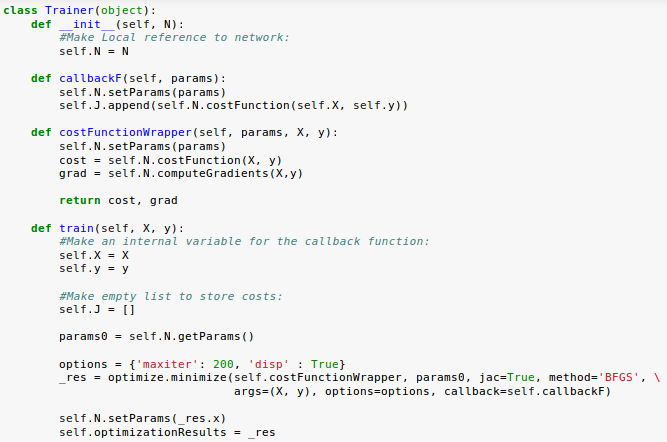
To use BFGS, the minimize function should have an objective function that accepts a vector of parameters, input data, and output data, and returns both the cost and gradients.
So, we're using a wrapper API around our ANN code. Also, we're implementing a callback function that allows us to track the cost function value as we train the network:
_res = optimize.minimize(self.costFunctionWrapper, params0, \
                         jac=True, method='BFGS', \
                         args=(X, y), options=options, \
                         callback=self.callbackF)
Note that we pass in initial parameters, set the jacobian parameter to true since we're computing the gradient within our neural network class, set the method to BFGS, pass in our input and output data.
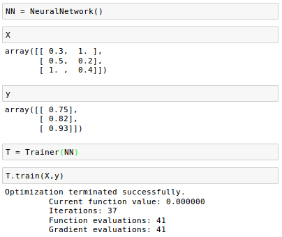
Let's train our neural network:
Plot the cost($J$) against the number of iterations through training:
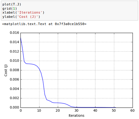
As we can see we have monotonically decreasing function.
Also, the number of iterations is less than 100, and much more efficient than the brute force algorithm we used in part 3.
Note that as we're approaching the solution, the curve becomes flatten and the gradient of $J$ gets smaller and smaller. We can check the values: $\frac {\partial J}{\partial W^{(1)}}$ and $\frac {\partial J}{\partial W^{(2)}}$:

Finally, we have a trained network that can predict our score on a test based on how many hours we sleep and how many hours we study the night before!
If we run our training data through our forward method (forwardPropagation().
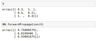
We can see that our predictions ($\hat y$) from forward method are pretty good compared with our target values ($y$).

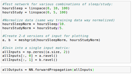
Now we can go one step further and explore the input space created from numpy's linspace for various combinations of hours sleeping and hours studying:
hoursSleep = linspace(0, 10, 100)
hoursStudy = linspace(0, 5, 100)
Here is our test code:
The plot looks like this:
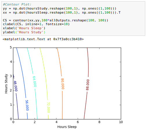
From the contour picture we may find an optimal combination of the two for our next test!
We can draw 3-D plot as well:
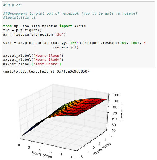
It looks like our sleep hours actually has a bigger impact on our grade than study hours!
Our trained neural network looks pretty good. However, it's not guaranteed that we get the quality results from real world data. That's because we used very small size training data. Even though we use lots of data set to train our model, it may be overfitted and may not give us the desired results for a new data set.
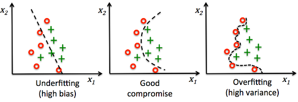
picture source : Python machine learning by Sebastian Raschka
So, in our next article, we'll deal with this issue.
Next:
7. Overfitting & RegularizationMachine Learning with scikit-learn
scikit-learn installation
scikit-learn : Features and feature extraction - iris dataset
scikit-learn : Machine Learning Quick Preview
scikit-learn : Data Preprocessing I - Missing / Categorical data
scikit-learn : Data Preprocessing II - Partitioning a dataset / Feature scaling / Feature Selection / Regularization
scikit-learn : Data Preprocessing III - Dimensionality reduction vis Sequential feature selection / Assessing feature importance via random forests
Data Compression via Dimensionality Reduction I - Principal component analysis (PCA)
scikit-learn : Data Compression via Dimensionality Reduction II - Linear Discriminant Analysis (LDA)
scikit-learn : Data Compression via Dimensionality Reduction III - Nonlinear mappings via kernel principal component (KPCA) analysis
scikit-learn : Logistic Regression, Overfitting & regularization
scikit-learn : Supervised Learning & Unsupervised Learning - e.g. Unsupervised PCA dimensionality reduction with iris dataset
scikit-learn : Unsupervised_Learning - KMeans clustering with iris dataset
scikit-learn : Linearly Separable Data - Linear Model & (Gaussian) radial basis function kernel (RBF kernel)
scikit-learn : Decision Tree Learning I - Entropy, Gini, and Information Gain
scikit-learn : Decision Tree Learning II - Constructing the Decision Tree
scikit-learn : Random Decision Forests Classification
scikit-learn : Support Vector Machines (SVM)
scikit-learn : Support Vector Machines (SVM) II
Flask with Embedded Machine Learning I : Serializing with pickle and DB setup
Flask with Embedded Machine Learning II : Basic Flask App
Flask with Embedded Machine Learning III : Embedding Classifier
Flask with Embedded Machine Learning IV : Deploy
Flask with Embedded Machine Learning V : Updating the classifier
scikit-learn : Sample of a spam comment filter using SVM - classifying a good one or a bad one
Machine learning algorithms and concepts
Batch gradient descent algorithmSingle Layer Neural Network - Perceptron model on the Iris dataset using Heaviside step activation function
Batch gradient descent versus stochastic gradient descent
Single Layer Neural Network - Adaptive Linear Neuron using linear (identity) activation function with batch gradient descent method
Single Layer Neural Network : Adaptive Linear Neuron using linear (identity) activation function with stochastic gradient descent (SGD)
Logistic Regression
VC (Vapnik-Chervonenkis) Dimension and Shatter
Bias-variance tradeoff
Maximum Likelihood Estimation (MLE)
Neural Networks with backpropagation for XOR using one hidden layer
minHash
tf-idf weight
Natural Language Processing (NLP): Sentiment Analysis I (IMDb & bag-of-words)
Natural Language Processing (NLP): Sentiment Analysis II (tokenization, stemming, and stop words)
Natural Language Processing (NLP): Sentiment Analysis III (training & cross validation)
Natural Language Processing (NLP): Sentiment Analysis IV (out-of-core)
Locality-Sensitive Hashing (LSH) using Cosine Distance (Cosine Similarity)
Artificial Neural Networks (ANN)
[Note] Sources are available at Github - Jupyter notebook files1. Introduction
2. Forward Propagation
3. Gradient Descent
4. Backpropagation of Errors
5. Checking gradient
6. Training via BFGS
7. Overfitting & Regularization
8. Deep Learning I : Image Recognition (Image uploading)
9. Deep Learning II : Image Recognition (Image classification)
10 - Deep Learning III : Deep Learning III : Theano, TensorFlow, and Keras
Ph.D. / Golden Gate Ave, San Francisco / Seoul National Univ / Carnegie Mellon / UC Berkeley / DevOps / Deep Learning / Visualization