Signal Processing with NumPy - Fourier Transform : FFT & DFT

A fast Fourier transform (FFT) is a method to calculate a discrete Fourier transform (DFT).
Spectral analysis is the process of determining the frequency domain representation of a signal in time domain and most commonly employs the Fourier transform. The Discrete Fourier Transform (DFT) is used to determine the frequency content of signals and the Fast Fourier Transform (FFT) is an efficient method for calculating the DFT.
Fourier analysis is fundamentally a method:
- To express a function as a sum of periodic components.
- To recover the function from those components.
"When both the function and its Fourier transform are replaced with discretized counterparts, it is called the discrete Fourier transform (DFT). The DFT has become a mainstay of numerical computing in part because of a very fast algorithm for computing it, called the Fast Fourier Transform (FFT), which was known to Gauss (1805) and was brought to light in its current form by Cooley and Tukey [CT]. Press et al. [NR] provide an accessible introduction to Fourier analysis and its applications." - from Discrete Fourier Transform
In this chapter, we can peek into the FFT/DFT via the examples for sine wave, square wave, and unit pulse.
import numpy as np
import matplotlib.pyplot as plt
from scipy import fft

Fs = 150                         # sampling rate
Ts = 1.0/Fs                      # sampling interval
t = np.arange(0,1,Ts)            # time vector
ff = 5                           # frequency of the signal
y = np.sin(2 * np.pi * ff * t)

plt.subplot(2,1,1)
plt.plot(t,y,'k-')
plt.xlabel('time')
plt.ylabel('amplitude')

plt.subplot(2,1,2)
n = len(y)                       # length of the signal
k = np.arange(n)
T = n/Fs
frq = k/T # two sides frequency range
freq = frq[range(n/2)]           # one side frequency range

Y = np.fft.fft(y)/n              # fft computing and normalization
Y = Y[range(n/2)]

plt.plot(freq, abs(Y), 'r-')
plt.xlabel('freq (Hz)')
plt.ylabel('|Y(freq)|')

plt.show()
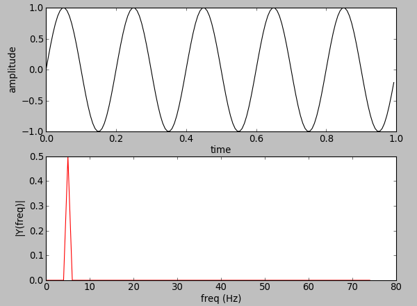
5 Hz sine wave:
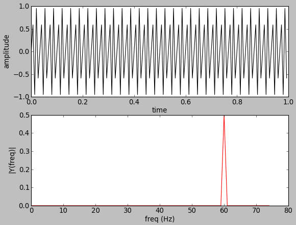
60 Hz sine wave:
import numpy as np
import matplotlib.pyplot as plt
from scipy import fft

Fs = 200                         # sampling rate
Ts = 1.0/Fs                      # sampling interval
t = np.arange(0,1,Ts)            # time vector
ff = 20                          # frequency of the signal

zero = np.zeros(10)
zeros = np.zeros(Fs/ff/2)
ones = np.ones(Fs/ff/2)
count = 0
y = []
for i in range(Fs):
    if i % Fs/ff/2 == 0:
        if count % 2 == 0:
            y = np.append(y,zeros)
        else:
            y = np.append(y,ones)
        count += 1

plt.subplot(2,1,1)
plt.plot(t,y,'k-')
plt.xlabel('time')
plt.ylabel('amplitude')

plt.subplot(2,1,2)
n = len(y)                       # length of the signal
k = np.arange(n)
T = n/Fs
frq = k/T # two sides frequency range
freq = frq[range(n/2)]           # one side frequency range

Y = np.fft.fft(y)/n              # fft computing and normalization
Y = Y[range(n/2)]

plt.plot(freq, abs(Y), 'r-')
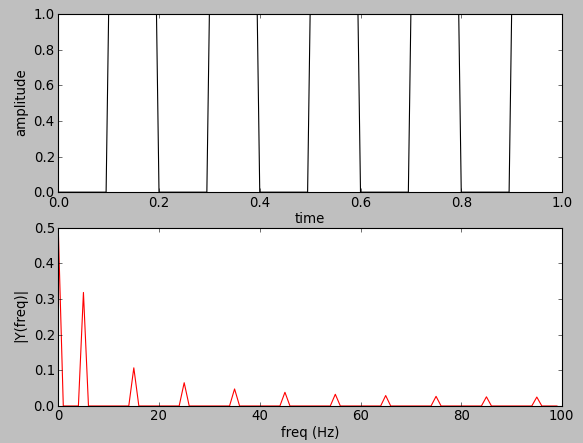
5 Hz square wave:
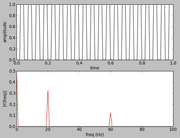
20 Hz square wave:
The code is almost identical to the previous codes except the pulse generation part:
import numpy as np
import matplotlib.pyplot as plt
from scipy import fft

Fs = 200                         # sampling rate
Ts = 1.0/Fs                      # sampling interval
t = np.arange(0,1,Ts)            # time vector
ff = 5                           # frequency of the signal

nPulse = 20
y = np.ones(nPulse)
y = np.append(y, np.zeros(Fs-nPulse))

plt.subplot(2,1,1)
plt.plot(t,y,'k-')
plt.xlabel('time')
plt.ylabel('amplitude')

plt.subplot(2,1,2)
n = len(y)                       # length of the signal
k = np.arange(n)
T = n/Fs
frq = k/T # two sides frequency range
freq = frq[range(n/2)]           # one side frequency range

Y = np.fft.fft(y)/n              # fft computing and normalization
Y = Y[range(n/2)]

plt.plot(freq, abs(Y), 'r-')
plt.xlabel('freq (Hz)')
plt.ylabel('|Y(freq)|')

plt.show()
Unit pulse:
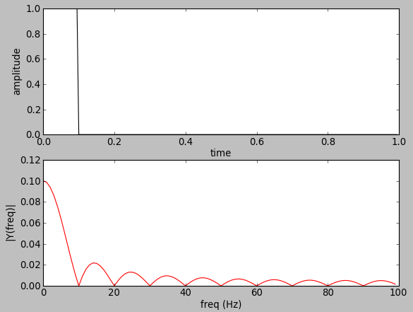
import numpy as np
import matplotlib.pyplot as plt
from scipy import fft

Fs = 200                         # sampling rate
Ts = 1.0/Fs                      # sampling interval
t = np.arange(0,1,Ts)            # time vector
ff = 5                           # frequency of the signal

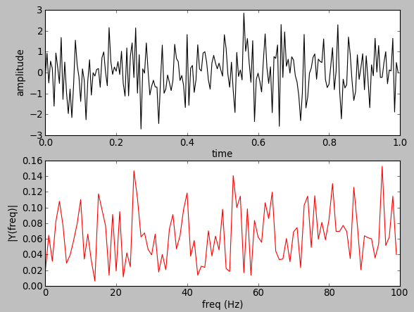
y = np.random.randn(Fs)

plt.subplot(2,1,1)
plt.plot(t,y,'k-')
plt.xlabel('time')
plt.ylabel('amplitude')

plt.subplot(2,1,2)
n = len(y)                       # length of the signal
k = np.arange(n)
T = n/Fs
frq = k/T # two sides frequency range
freq = frq[range(n/2)]           # one side frequency range

Y = np.fft.fft(y)/n              # fft computing and normalization
Y = Y[range(n/2)]

plt.plot(freq, abs(Y), 'r-')
plt.xlabel('freq (Hz)')
plt.ylabel('|Y(freq)|')

plt.show()
OpenCV 3 Tutorial
image & video processing
Installing on Ubuntu 13
Mat(rix) object (Image Container)
Creating Mat objects
The core : Image - load, convert, and save
Smoothing Filters A - Average, Gaussian
Smoothing Filters B - Median, Bilateral
OpenCV 3 image and video processing with Python
OpenCV 3 with Python
Image - OpenCV BGR : Matplotlib RGB
Basic image operations - pixel access
iPython - Signal Processing with NumPy
Signal Processing with NumPy I - FFT and DFT for sine, square waves, unitpulse, and random signal
Signal Processing with NumPy II - Image Fourier Transform : FFT & DFT
Inverse Fourier Transform of an Image with low pass filter: cv2.idft()
Image Histogram
Video Capture and Switching colorspaces - RGB / HSV
Adaptive Thresholding - Otsu's clustering-based image thresholding
Edge Detection - Sobel and Laplacian Kernels
Canny Edge Detection
Hough Transform - Circles
Watershed Algorithm : Marker-based Segmentation I
Watershed Algorithm : Marker-based Segmentation II
Image noise reduction : Non-local Means denoising algorithm
Image object detection : Face detection using Haar Cascade Classifiers
Image segmentation - Foreground extraction Grabcut algorithm based on graph cuts
Image Reconstruction - Inpainting (Interpolation) - Fast Marching Methods
Video : Mean shift object tracking
Machine Learning : Clustering - K-Means clustering I
Machine Learning : Clustering - K-Means clustering II
Machine Learning : Classification - k-nearest neighbors (k-NN) algorithm
Ph.D. / Golden Gate Ave, San Francisco / Seoul National Univ / Carnegie Mellon / UC Berkeley / DevOps / Deep Learning / Visualization