Image Fourier Transform : OpenCV FFT & DFT

In previous chapters, we looked into how we can use FFT and DFT in NumPy:
- OpenCV 3 iPython - Signal Processing with NumPy
- OpenCV 3 Signal Processing with NumPy I - FFT & DFT for sine, square waves, unitpulse, and random signal
- OpenCV 3 Signal Processing with NumPy II - Image Fourier Transform : FFT & DFT
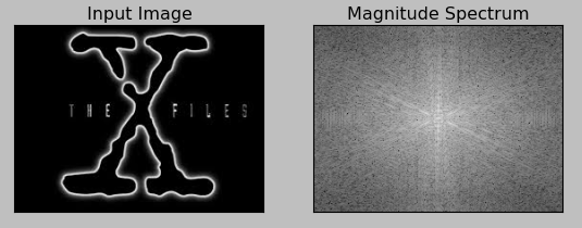
OpenCV has cv2.dft() and cv2.idft() functions, and we get the same result as with NumPy. OpenCV provides us two channels:
- The first channel represents the real part of the result.
- The second channel for the imaginary part of the result.
So, the shape of the returned np.ndarray from the functions will be (rows, cols, 2).
import numpy as np
import cv2
from matplotlib import pyplot as plt

img = cv2.imread('xfiles.jpg',0)

img_float32 = np.float32(img)

dft = cv2.dft(img_float32, flags = cv2.DFT_COMPLEX_OUTPUT)
dft_shift = np.fft.fftshift(dft)

magnitude_spectrum = 20*np.log(cv2.magnitude(dft_shift[:,:,0],dft_shift[:,:,1]))

plt.subplot(121),plt.imshow(img, cmap = 'gray')
plt.title('Input Image'), plt.xticks([]), plt.yticks([])
plt.subplot(122),plt.imshow(magnitude_spectrum, cmap = 'gray')
plt.title('Magnitude Spectrum'), plt.xticks([]), plt.yticks([])
plt.show()

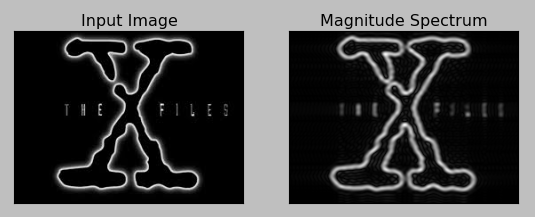
In this section, we'll create a LPF to remove high frequency contents in the image. In other words, we're going to apply LPF to the image which has blurring effect.
import numpy as np
import cv2
from matplotlib import pyplot as plt

img = cv2.imread('xfiles.jpg',0)

img_float32 = np.float32(img)

dft = cv2.dft(img_float32, flags = cv2.DFT_COMPLEX_OUTPUT)
dft_shift = np.fft.fftshift(dft)

rows, cols = img.shape
crow, ccol = rows/2 , cols/2     # center

# create a mask first, center square is 1, remaining all zeros
mask = np.zeros((rows, cols, 2), np.uint8)
mask[crow-30:crow+30, ccol-30:ccol+30] = 1

# apply mask and inverse DFT
fshift = dft_shift*mask
f_ishift = np.fft.ifftshift(fshift)
img_back = cv2.idft(f_ishift)
img_back = cv2.magnitude(img_back[:,:,0],img_back[:,:,1])

plt.subplot(121),plt.imshow(img, cmap = 'gray')
plt.title('Input Image'), plt.xticks([]), plt.yticks([])
plt.subplot(122),plt.imshow(img_back, cmap = 'gray')
plt.title('Magnitude Spectrum'), plt.xticks([]), plt.yticks([])

plt.show()
To apply Low Pass Filter (LPF), we create a mask first with high value (1) at low frequencies, and 0 at HF region.
mask = np.zeros((rows,cols,2), np.uint8)
mask[crow-30:crow+30, ccol-30:ccol+30] = 1
Note that the the mask.shape is (rows, cols, 2) which matches the returned np.ndarray from cv2.dft().
Also, unlike we've done in previous chapter (OpenCV 3 Signal Processing with NumPy II - Image Fourier Transform : FFT & DFT), we're applying LPF to the center's DC component.

As we discussed earlier, since we passed low frequencies, we see the image is blurred.
"OpenCV functions cv2.dft() and cv2.idft() are faster than Numpy counterparts. But Numpy functions are more user-friendly." - from Fourier Transform - OpenCV 3.0.0-dev documentation.
Ph.D. / Golden Gate Ave, San Francisco / Seoul National Univ / Carnegie Mellon / UC Berkeley / DevOps / Deep Learning / Visualization